8.3: Cutting Models

Figure 8-18: The Crushed Type.

Figure 8-19: The Chip Type.

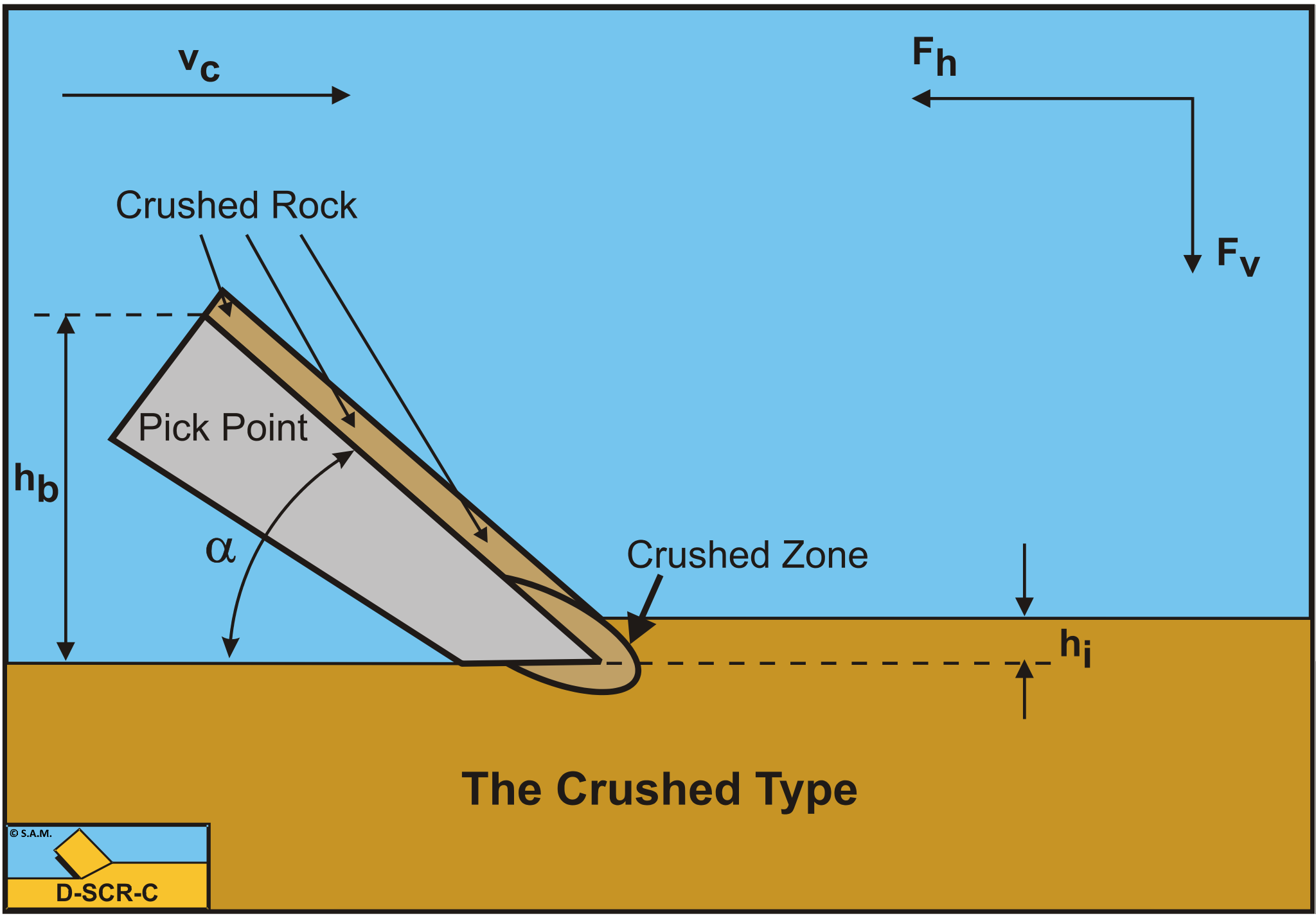
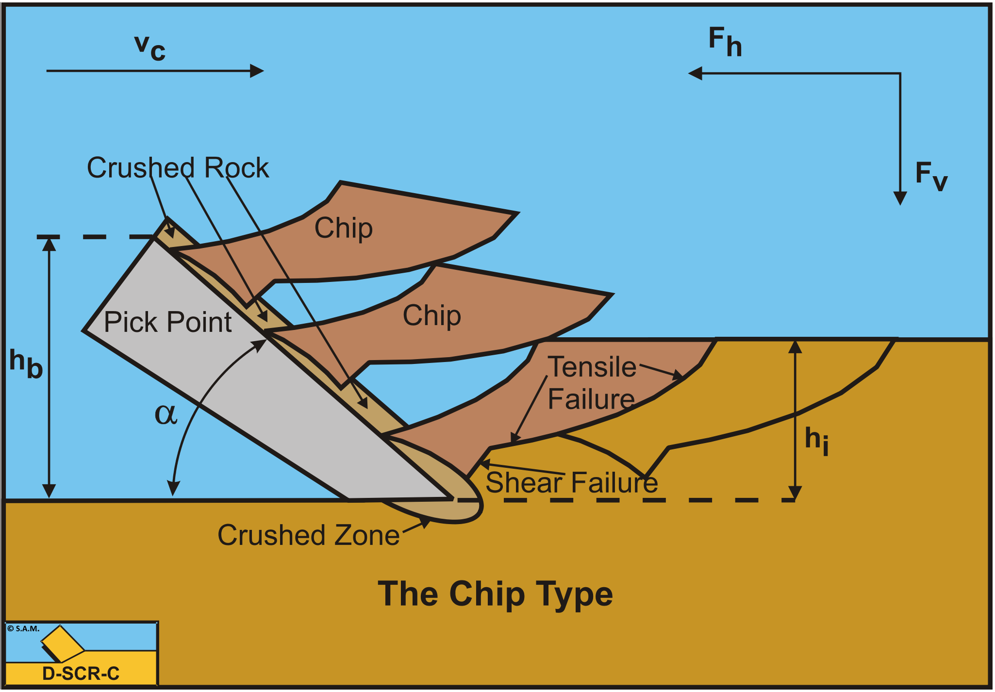
When cutting rock with a pick point, usually a crushed zone will occur in front of and under the tip of the pick point. If the cutting depth is small, this crushed zone may reach the surface and a sand like cutting process may occur. If the cutting depth is larger, the crushed material cannot escape and the stresses in the crushed zone increase strongly. According to Fairhurst (1964) the cutting forces are transmitted through particle-particle contacts. The stresses are transmitted to the intact rock as discrete point loads this way, causing micro shear cracks and finally a tensile crack. Figure 8-18 and Figure 8-19 sho this cutting mechanism.

As mentioned the type of failure depends on the UCS/BTS ratio. Geking (1987) stated that below a ratio of 9 ductile failure will occur, while above a ratio of 15 brittle failure will occur. In between these limits there is a transition between ductile and brittle failure, which is also in accordance with the findings of Fairhurst (1964). The mechanism as described above is difficult to model. Still a method is desired to predict the cutting forces in rock cutting in order to estimate forces, power and production. In literature some models exist, like the Evans (1964) model based on tensile failure and the Nishimatsu (1972) model based on shear failure. From steel cutting also the Merchant (1944) model is known, based on plastic shear failure. The Evans (1964) model assumes a maximum tensile stress on the entire failure plane, which could match the peak forces, but overestimates the average forces. Nishimatsu (1972) build in a factor for the shear stress distribution on the failure plane, enabling the model to take into account that failure may start when the shear stress is not at a maximum everywhere in the shear plane. Both models are discussed in this chapter.

Based on the Merchant (1944) model for steel cutting and the Miedema (1987 September) model for sand cutting, a new model is developed, both for ductile cutting, ductile cataclastic cutting, brittle shear cutting and brittle tensile cutting. First a model is derived for the Flow Type, which is either ductile shear failure or brittle shear failure. In the case of brittle shear failure, the maximum cutting forces are calculated. For the average cutting forces the maximum cutting forces have to be reduced by 30% to 50%. Based on the Flow Type and the Mohr circle, the shear stress in the shear plane is determined where, on another plane (direction), tensile stresses occur equal to the tensile strength. An equivalent or mobilized shear strength is determined giving this tensile stress, leading to the Tear Type of failure. This approach does not require the tensile stress to be equal to the tensile strength on the whole failure plane, instead it predicts the cutting forces at the start of tensile failure.

This method can also be used for predicting the cutting forces in frozen clay, permafrost.

Roxborough (1987) derived a simple expression for the specific energy based on many experiments in different types of rock. The dimension of this equation is MPa. The two constants in the equation may vary a bit depending on the type of rock. The 0.11 is important at small UCS values, the 0.25 at large values.

\[\ \mathrm{E}_{\mathrm{sp}}=\mathrm{0 .2 5} \cdot \mathrm{U.C.S.}+\mathrm{0.11}\tag{8-40}\]

The fact that cutting rock is irreversible, compared to the cutting of sand and clay, also means that the 4 standard cutting mechanisms cannot be applied on cutting rock. In fact the Flow Type looks like cataclastic ductile failure from a macroscopic point of view, but the Flow Type (also the Curling Type) are supposed to be real plastic deformation after which the material (clay) is still in tact, while cataclastic ductile failure is much more the crushing of the rock with shear falure in the crushed rock. We will name this the Crushed Type. When the layer cut is thicker, a crushed zone exists but not to the free surface. From the crushed zone first a shear plane is formed from which a tensile crack goes to the free surface. We will name this the Chip Type.

8.3.1. The Model of Evans

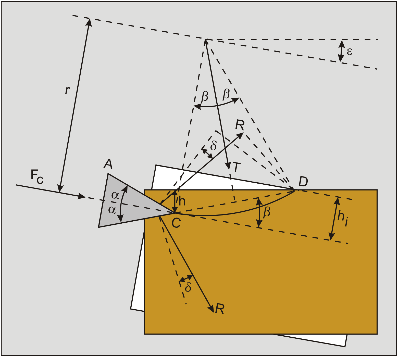
For brittle rock the cutting theory of Evans (1964) and (1966) can be used to calculate cutting forces (Figure 8-21). The forces are derived from the geometry of the chisel (width, cutting angle and cutting depth) and the tensile strength (BTS) of the rock. Evans suggested a model on basis of observations on coal breakage by wedges. In this theory it is assumed that:

1. A force R is acting under an angle δ (external friction angle) with the normal to the surface A-C of the wedge.

2. A resultant force T of the tensile stresses acting at the center of the arc C-D, the line C-D is under an angle β (the shear angle) with the horizontal.

3. A third force S is required to maintain equilibrium in the buttock, but does not play a role in the derivation.

4. The penetration of the wedge is small compared to the layer thickness h_i.

The action of the wedge tends to split the rock and does rotate it about point D. It is therefore assumed that the force S acts through point D. Along the fracture line, it is assumed that a state of plain strain is working and the equilibrium is considered per unit of width w of the wedge.

\[\ \mathrm{\mathrm{T}=\sigma_{\mathrm{T}} \cdot \mathrm{r} \cdot \int_{-\beta}^{\beta} \cos (\omega) \cdot \mathrm{d} \omega \cdot \mathrm{w}=2 \cdot \sigma_{T} \cdot \mathrm{r} \cdot \sin (\beta) \cdot \mathrm{w}}\tag{8-41}\]

Where r·dω is an element of the arc C-D making an angle ω with the symmetry axis of the arc. Let h_i be the depth of the cut and assume that the penetration of the edge may be neglected in comparison with h_i. This means that the force R is acting near point C. Taking moments on the chip cut about point D gives:

\[\ \mathrm{R} \cdot \cos (\alpha+\beta+\delta) \cdot \frac{\mathrm{h}_{\mathrm{i}}}{\sin (\beta)}=\mathrm{T} \cdot \mathrm{r} \cdot \sin (\beta)=2 \cdot \sigma_{\mathrm{T}} \cdot \mathrm{r} \cdot \sin (\beta) \cdot \mathrm{w} \cdot \mathrm{r} \cdot \sin (\beta)\tag{8-42}\]

From the geometric relation it follows:

\[\ \mathrm{r} \cdot \sin (\beta)=\frac{\mathrm{h}_{\mathrm{i}}}{2 \cdot \sin (\beta)}\tag{8-43}\]

Hence:

\[\ \mathrm{R}=\frac{\sigma_{\mathrm{T}} \cdot \mathrm{h}_{\mathrm{i}} \cdot \mathrm{w}}{2 \cdot \sin (\beta) \cdot \cos (\alpha+\beta+\delta)}\tag{8-44}\]

The horizontal component of R is R·sin(α+δ) and due to the symmetry of the forces acting on the wedge the total cutting force is:

\[\ \mathrm{F}_{\mathrm{c}}=\mathrm{2} \cdot \mathrm{R} \cdot \sin (\alpha+\delta)=\sigma_{\mathrm{T}} \cdot \mathrm{h}_{\mathrm{i}} \cdot \mathrm{w} \cdot \frac{\sin (\alpha+\delta)}{\sin (\beta) \cdot \cos (\alpha+\beta+\delta)}\tag{8-45}\]

The normal force (\(\ \perp\) on cutting force) is per side:

\[\ \mathrm{F}_{\mathrm{n}}=\mathrm{R} \cdot \cos (\alpha+\delta)=\sigma_{\mathrm{T}} \cdot \mathrm{h}_{\mathrm{i}} \cdot \mathrm{w} \cdot \frac{\cos (\alpha+\delta)}{2 \cdot \sin (\beta) \cdot \cos (\alpha+\beta+\delta)}\tag{8-46}\]

The angle β can be determined by using the principle of minimum energy:

\[\ \frac{\mathrm{d} \mathrm{F}_{\mathrm{c}}}{\mathrm{d} \beta}=0\tag{8-47}\]

Giving:

\[\ \begin{array}{left}\cos (\beta) \cdot \cos (\alpha+\beta+\delta)-\sin (\beta) \cdot \sin (\alpha+\beta+\delta)=0\\
\Rightarrow \cos (2 \cdot \beta+\alpha+\delta)=0\end{array}\tag{8-48}\]

Resulting in:

\[\ \beta=\frac{1}{2} \cdot\left(\frac{\pi}{2}-\alpha-\delta\right)=\frac{\pi}{4}-\frac{\alpha+\delta}{2}\tag{8-49}\]

With:

\[\ \sin (\beta) \cdot \cos (\alpha+\beta+\delta)=\frac{1-\sin (\alpha+\delta)}{2}\tag{8-50}\]

This gives for the horizontal cutting force:

\[\ \mathrm{F}_{\mathrm{c}}=\sigma_{\mathrm{T}} \cdot \mathrm{h}_{\mathrm{i}} \cdot \mathrm{w} \cdot \frac{\mathrm{2} \cdot \sin (\alpha+\delta)}{1-\sin (\alpha+\delta)}=\sigma_{\mathrm{T}} \cdot \mathrm{h}_{\mathrm{i}} \cdot \mathrm{w} \cdot \lambda_{\mathrm{H T}}\tag{8-51}\]

For each side of the wedge the normal force is now (the total normal/vertical force is zero):

\[\ \mathrm{F}_{\mathrm{n}}=\sigma_{\mathrm{T}} \cdot \mathrm{h}_{\mathrm{i}} \cdot \mathrm{w} \cdot \frac{\cos (\alpha+\delta)}{1-\sin (\alpha+\delta)}=\sigma_{\mathrm{T}} \cdot \mathrm{h}_{\mathrm{i}} \cdot \mathrm{w} \cdot \lambda_{\mathrm{V T}}\tag{8-52}\]

Figure 8-20: The brittle-tear horizontal force coefficient λ_HT (Evans).

Figure 8-21: The model of Evans.

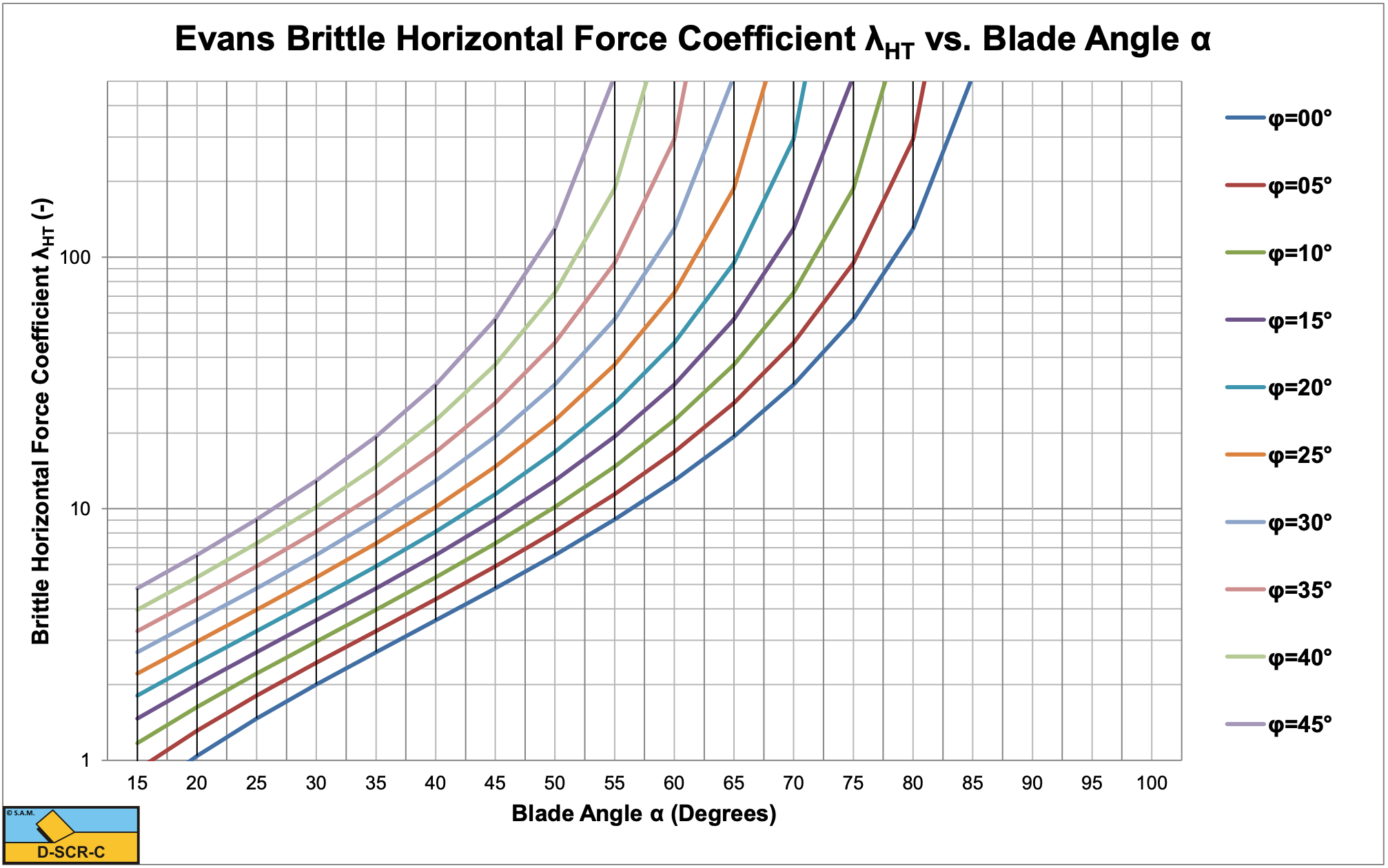
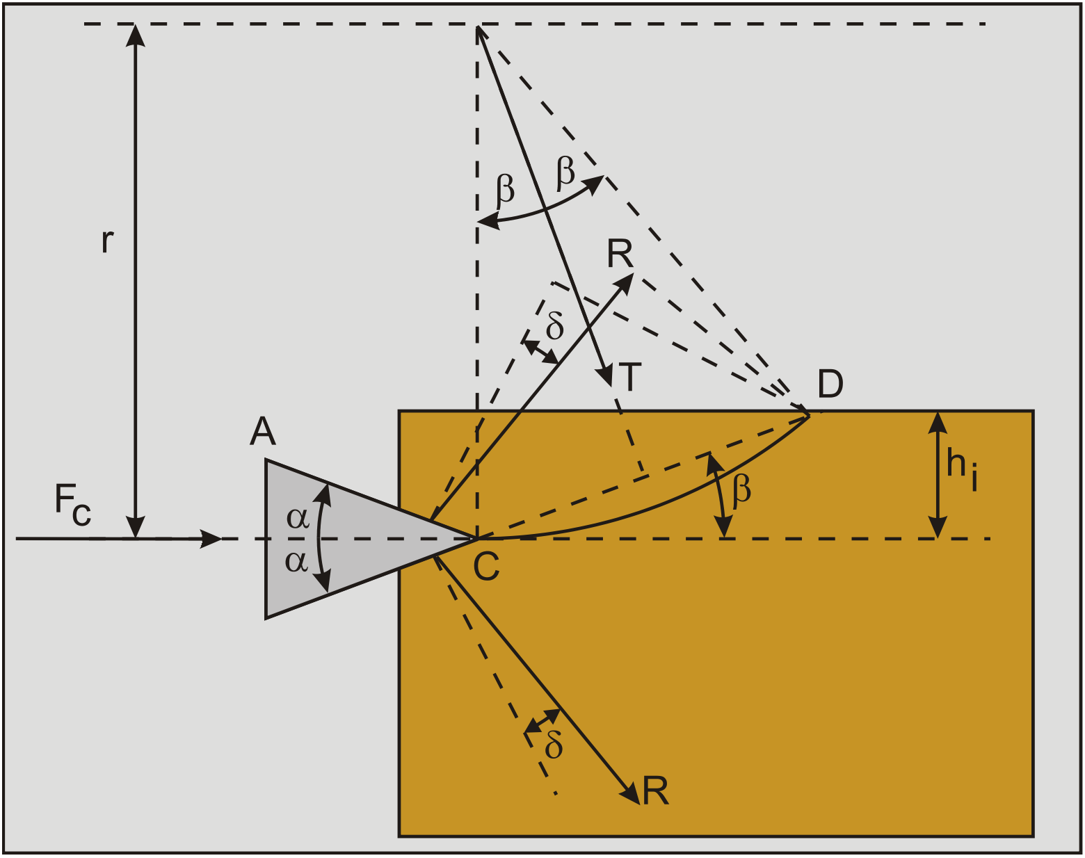
Figure 8-20 shows the brittle-tear horizontal force coefficient λ_HT as a function of the wedge top angle α and the internal friction angle φ. The internal friction angle φ does not play a role directly, but it is assumed that the external friction angle δ is 2/3 of the internal friction angle φ. Comparing Figure 8-20 with Figure 8-42 (the brittle- tear horizontal force coefficient λ_HT of the Miedema model) shows that the coefficient λ_HT of Evans is bigger than the λ_HT coefficient of Miedema. The Miedema model however is based on cutting with a blade, while Evans is based on the penetration with a wedge or chisel, which should give a higher cutting force. The model as is derived in chapter 8.3 assumes sharp blades however. 

8.3.2. The Model of Evans under an Angle ε

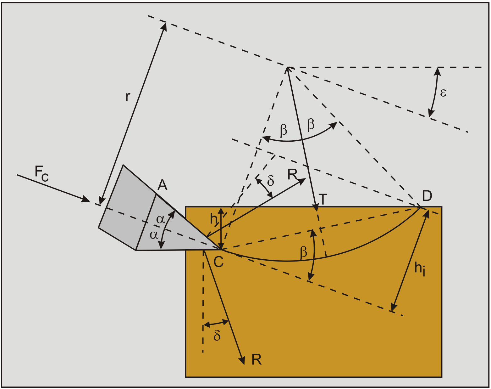
When it is assumed that the chisel enters the rock under an angle ε and the fracture starts in the same direction as the centerline of the chisel as is shown in Figure 8-22, the following can be derived:

\[\ \mathrm{h}=\mathrm{2} \cdot \mathrm{r} \cdot \sin (\beta) \cdot \sin (\beta-\varepsilon)\text{ and }\mathrm{h}_{\mathrm{i}}=2 \cdot \mathrm{r} \cdot \sin ^{2}(\beta)\tag{8-53}\]

\[\ \mathrm{h_{i}=h \cdot \frac{\sin (\beta)}{\sin (\beta-\varepsilon)}}\tag{8-54}\]

Substituting equation (8-53) in equation (8-45) for the cutting force gives:

\[\ \begin{array}{left} \mathrm{F}_{\mathrm{c}}&= \sigma_{\mathrm{T}} \cdot \mathrm{h}_{\mathrm{i}} \cdot \mathrm{w} \cdot \frac{\mathrm{2} \cdot \mathrm{s i n}(\boldsymbol{\alpha}+\delta)}{\mathrm{1}-\sin (\alpha+\delta)} \\&= \sigma_{\mathrm{T}} \cdot \mathrm{h} \cdot \mathrm{w} \cdot \frac{\sin (\beta)}{\sin (\beta-\varepsilon)} \cdot \frac{\sin (\alpha+\delta)}{\sin (\beta) \cdot \cos (\alpha+\beta+\delta)} \\&= \sigma_{T} \cdot \mathrm{h} \cdot \mathrm{w} \cdot \frac{\sin (\alpha+\delta)}{\sin (\beta-\varepsilon) \cdot \cos (\alpha+\beta+\delta)} \end{array}\tag{8-55}\]

The horizontal component of the cutting force is now:

\[\ \mathrm{F_{\mathrm{ch}}=\sigma_{\mathrm{T}} \cdot h \cdot \mathrm{w} \cdot \frac{\sin (\alpha+\delta)}{\sin (\beta-\varepsilon) \cdot \cos (\alpha+\beta+\delta)} \cdot \cos (\varepsilon)}\tag{8-56}\]

The vertical component of this cutting force is now:

\[\ \mathrm{F}_{\mathrm{cv}}=\sigma_{\mathrm{T}} \cdot \mathrm{h} \cdot \mathrm{w} \cdot \frac{\sin (\alpha+\delta)}{\sin (\beta-\varepsilon) \cdot \cos (\alpha+\beta+\delta)} \cdot \sin (\varepsilon)\tag{8-57}\]

Note that the vertical force is not zero anymore, which makes sense since the chisel is not symmetrical with regard to the horizontal anymore. Equation (8-58) can be applied to eliminate the shear angle β from the above equations. When the denominator is at a maximum in these equations, the forces are at a minimum. The denominator is at a maximum when the first derivative of the denominator is zero and the second derivative is negative.

Figure 8-22: The model of Evans under an angle ε.

The angle β can be determined by using the principle of minimum energy:

\[\ \frac{\mathrm{d} \mathrm{F}_{\mathrm{c}}}{\mathrm{d} \boldsymbol{\beta}}=\mathrm{0}\tag{8-58}\]

Giving for the first derivative:

\[\ \begin{array}{left} \cos (\beta-\varepsilon) \cdot \cos (\alpha+\beta+\delta)-\sin (\beta-\varepsilon) \cdot \sin (\alpha+\beta+\delta)=0\\
\Rightarrow \cos (2 \cdot \beta+\alpha+\delta-\varepsilon)=0\end{array}\tag{8-59}\]

Resulting in:

\[\ \beta=\frac{1}{2} \cdot\left(\frac{\pi}{2}-\alpha-\delta+\varepsilon\right)=\frac{\pi}{4}-\frac{\alpha+\delta-\varepsilon}{2}\tag{8-60}\]

With:

\[\ \sin (\beta-\varepsilon) \cdot \cos (\alpha+\beta+\delta)=\frac{1-\sin (\alpha+\delta+\varepsilon)}{2}\tag{8-61}\]

Substituting equation (8-61) in equation (8-55) gives for the force F_c:

\[\ \mathrm{F_{c}=\sigma_{T} \cdot h \cdot w \cdot \frac{2 \cdot \sin (\alpha+\delta)}{1-\sin (\alpha+\delta+\varepsilon)}}\tag{8-62}\]

The horizontal component of the cutting force F_ch is now:

\[\ \mathrm{F_{c h}=\sigma_{T} \cdot h \cdot w \cdot \frac{2 \cdot \sin (\alpha+\delta)}{1-\sin (\alpha+\delta+\varepsilon)} \cdot \cos (\varepsilon)}\tag{8-63}\]

The vertical component of this cutting force F_cv is now:

\[\ \mathrm{F_{c v}=\sigma_{T} \cdot h \cdot w \cdot \frac{2 \cdot \sin (\alpha+\delta)}{1-\sin (\alpha+\delta+\varepsilon)} \cdot \sin (\varepsilon)}\tag{8-64}\]

8.3.3. The Model of Evans used for a Pick point

In the case where the angle ε equals the angle α, a pick point with blade angle 2·α and a wear flat can be simulated as is shown in Figure 8-23. In this case the equations become:

\[\ \mathrm{F_{c}=\sigma_{T} \cdot h \cdot w \cdot \frac{2 \cdot \sin (\alpha+\delta)}{1-\sin (2 \cdot \alpha+\delta)}}\tag{8-65}\]

The horizontal component of the cutting force F_ch is now:

\[\ \mathrm{F_{c h}=\sigma_{T} \cdot h \cdot w \cdot \frac{2 \cdot \sin (\alpha+\delta)}{1-\sin (2 \cdot \alpha+\delta)} \cdot \cos (\alpha)}\tag{8-66}\]

The vertical component of this cutting force F_cv is now:

\[\ \mathrm{F_{c v}=\sigma_{T} \cdot h \cdot w \cdot \frac{2 \cdot \sin (\alpha+\delta)}{1-\sin (2 \cdot \alpha+\delta)} \cdot \sin (\alpha)}\tag{8-67}\]

For the force R (see equation (8-45)), acting on both sides of the pick point the following equation can be found:

\[\ \mathrm{R}=\frac{\mathrm{F}_{\mathrm{c}}}{\mathrm{2} \cdot \sin (\alpha+\delta)}=\sigma_{\mathrm{T}} \cdot \mathrm{h} \cdot \mathrm{w} \cdot \frac{\mathrm{1}}{1-\sin (2 \cdot \alpha+\delta)}\tag{8-68}\]

In the case of wear calculations the normal and friction forces on the front side and the wear flat can be interesting. According to Evans the normal and friction forces are the same on both sides, since this was the starting point of the derivation, this gives for the normal force R_n:

\[\ \mathrm{R_{n}=\sigma_{T} \cdot h \cdot w \cdot \frac{1}{1-\sin (2 \cdot \alpha+\delta)} \cdot \cos (\delta)}\tag{8-69}\]

The friction force R_f is now:

\[\ \mathrm{R}_{\mathrm{f}}=\sigma_{\mathrm{T}} \cdot \mathrm{h} \cdot \mathrm{w} \cdot \frac{\mathrm{1}}{1-\sin (2 \cdot \alpha+\delta)} \cdot \sin (\delta)\tag{8-70}\]

Figure 8-23: The model of Evans used for a pick point.

8.3.4. Summary of the Evans Theory

The Evans theory has been derived for 3 cases:

1. The basic case with a horizontal moving chisel and the centerline of the chisel horizontal.

2. A horizontal moving chisel with the centerline under an angle ε.

3. A pick point with the centerline angle ε equal to half the top angle α, horizontally moving.

Once again it should be noted that the angle α as used by Evans is half the top angle of the chisel and not the blade angle as α is used for in most equations in this book. In case 1 the blade angle would be α as used by Evans, in case 2 the blade angle is α+ε and in case 3 the blade angle is 2·α. In all cases it is assumed that the cutting velocity v_c is horizontal.

Table 8-2: Summary of the Evans theory.

Case	Cutting forces and specific energy
1	\[\ \begin{array}{left}\mathrm{F_{c}=\sigma_{T} \cdot h_{i} \cdot w \cdot \frac{2 \cdot \sin (\alpha+\delta)}{1-\sin (\alpha+\delta)}}\\ \mathrm{F_{c h}=F_{c}}\\ \mathrm{F_{c v}=0}\\ \mathrm{E_{s p}=\frac{F_{c h} \cdot v_{c}}{h_{i} \cdot w \cdot v_{c}}=\sigma_{T} \cdot \frac{2 \cdot \sin (\alpha+\delta)}{1-\sin (\alpha+\delta)}}\end{array}\tag{8-71}\]
2	\[\ \begin{array}{left}\mathrm{F}_{\mathrm{c}}=\sigma_{\mathrm{T}} \cdot \mathrm{h} \cdot \mathrm{w} \cdot \frac{\mathrm{2} \cdot \sin (\alpha+\delta)}{1-\sin (\alpha+\delta+\varepsilon)}\\ \mathrm{F}_{\mathrm{c h}}=\mathrm{F}_{\mathrm{c}} \cdot \cos (\varepsilon)\\ \mathrm{F}_{\mathrm{c v}}=\mathrm{F}_{\mathrm{c}} \cdot \sin (\varepsilon)\\ \mathrm{E}_{\mathrm{sp}}=\frac{\mathrm{F}_{\mathrm{c h}} \cdot \mathrm{v}_{\mathrm{c}}}{\mathrm{h}_{\mathrm{i}} \cdot \mathrm{w} \cdot \mathrm{v}_{\mathrm{c}}}=\sigma_{\mathrm{T}} \cdot \frac{\mathrm{2} \cdot \sin (\alpha+\delta)}{1-\sin (\alpha+\delta+\varepsilon)} \cdot \cos (\varepsilon)\end{array}\tag{8-72}\]
3	\[\ \begin{array}{left}\mathrm{F}_{\mathrm{c}}=\sigma_{\mathrm{T}} \cdot \mathrm{h} \cdot \mathrm{w} \cdot \frac{\mathrm{2} \cdot \sin (\alpha+\delta)}{1-\sin (\mathrm{2} \cdot \alpha+\delta)}\\ \mathrm{F}_{\mathrm{c h}}=\mathrm{F}_{\mathrm{c}} \cdot \cos (\alpha)\\ \mathrm{F}_{\mathrm{c v}}=\mathrm{F}_{\mathrm{c}} \cdot \sin (\alpha)\\ \mathrm{E}_{\mathrm{sp}}=\frac{\mathrm{F}_{\mathrm{c h}} \cdot \mathrm{v}_{\mathrm{c}}}{\mathrm{h}_{\mathrm{i}} \cdot \mathrm{w} \cdot \mathrm{v}_{\mathrm{c}}}=\sigma_{\mathrm{T}} \cdot \frac{\mathrm{2} \cdot \sin (\alpha+\delta)}{1-\sin (2 \cdot \alpha+\delta)} \cdot \cos (\alpha)\end{array}\tag{8-73}\]

8.3.5. The Nishimatsu Model

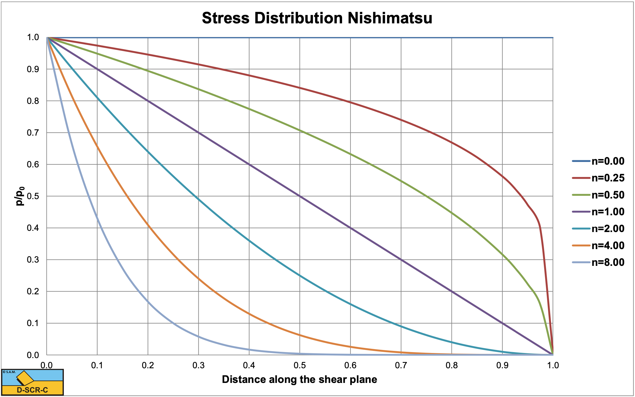
For brittle shear rock cutting we may use the equation of Nishimatsu (1972). This theory describes the cutting force of chisels by failure through shear. Figure 8-24 gives the parameters needed to calculate the cutting forces. Nishimatsu (1972) presented a theory similar to Merchant ́s (1944), (1945A) and (1945B) only Nishimatsu’s theory considered the normal and shear stresses acting on the failure plain (A-B) to be proportional to the n^th power of the distance λ from point A to point B. With n being the so called stress distribution factor:

\[\ \mathrm{p}=\mathrm{p}_{0} \cdot\left(\frac{\mathrm{h}_{\mathrm{i}}}{\sin (\beta)}-\lambda\right)^{\mathrm{n}}\tag{8-74}\]

Nishumatsu made the following assumptions:

1. The rock cutting is brittle, without any accompanying plastic deformation (no ductile crushing zone).

2. The cutting process is under plain stress condition.

3. The failure is according a linear Mohr envelope.

4. The cutting speed has no effect on the processes.

Figure 8-24: Model for shear failure by Nishimatsu (1972).

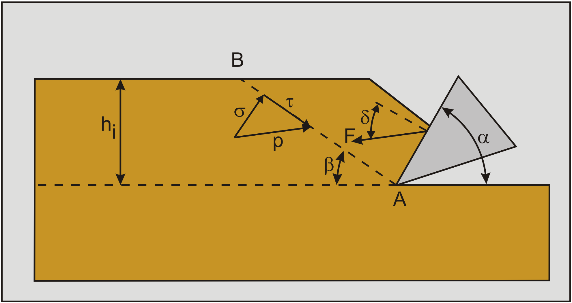
As a next assumption, let us assume that the direction of the resultant stress p is constant along the line A-B. The integration of this resultant stress p along the line A-B should be in equilibrium with the resultant cutting force F. Thus, we have:

\[\ \mathrm{p}_{0} \cdot \mathrm{w} \cdot \int_{0}^{\frac{\mathrm{h}_{\mathrm{i}}}{\sin (\beta)}}\left(\frac{\mathrm{h}_{\mathrm{i}}}{\sin (\beta)}-\lambda\right)^{\mathrm{n}} \cdot \mathrm{d} \lambda=\mathrm{F} \Rightarrow \mathrm{p}_{0} \cdot \mathrm{w} \cdot \frac{\mathrm{1}}{\mathrm{n}+\mathrm{1}} \cdot\left(\frac{\mathrm{h}_{\mathrm{i}}}{\sin (\beta)}\right)^{\mathrm{n}+1}=\mathrm{F}\tag{8-75}\]

Integrating the second term of equation (8-75) allows determining the value of the constant p₀.

\[\ \mathrm{p}_{0} \cdot \mathrm{w}=(\mathrm{n}+\mathrm{1}) \cdot\left(\frac{\mathrm{h}_{\mathrm{i}}}{\sin (\beta)}\right)^{-(\mathrm{n}+1)} \cdot \mathrm{F}\tag{8-76}\]

Substituting this in equation (8-74) gives:

\[\ \mathrm{p} \cdot \mathrm{w}=(\mathrm{n}+\mathrm{1}) \cdot\left(\frac{\mathrm{h}_{\mathrm{i}}}{\sin (\beta)}\right)^{-(\mathrm{n}+1)} \cdot\left(\frac{\mathrm{h}_{\mathrm{i}}}{\sin (\beta)}-\lambda\right)^{\mathrm{n}} \cdot \mathrm{F}\tag{8-77}\]

The maximum stress p is assumed to occur near the tip of the chisel, so λ=0, giving:

\[\ \mathrm{p} \cdot \mathrm{w}=(\mathrm{n}+\mathrm{1}) \cdot\left(\frac{\mathrm{h}_{\mathrm{i}}}{\sin (\beta)}\right)^{-1} \cdot \mathrm{F}\tag{8-78}\]

For the normal stress σ and the shear \(\ \tau\) stress this gives:

\[\ \sigma_{0} \cdot \mathrm{w}=-\mathrm{p} \cdot \mathrm{w} \cdot \cos (\alpha+\beta+\delta)=(\mathrm{n}+1) \cdot\left(\frac{\mathrm{h}_{\mathrm{i}}}{\sin (\beta)}\right)^{-1} \cdot \mathrm{F} \cdot \cos (\alpha+\beta+\delta)\tag{8-79}\]

\[\ \tau_{0} \cdot \mathrm{w}=\mathrm{p} \cdot \mathrm{w} \cdot \sin (\alpha+\beta+\delta)=(\mathrm{n}+1) \cdot\left(\frac{\mathrm{h}_{\mathrm{i}}}{\sin (\beta)}\right)^{-1} \cdot \mathrm{F} \cdot \sin (\alpha+\beta+\delta)\tag{8-80}\]

Rewriting this gives:

\[\ \sigma_{0} \cdot \mathrm{h}_{\mathrm{i}} \cdot \mathrm{w}=-\mathrm{p} \cdot \mathrm{h}_{\mathrm{i}} \cdot \mathrm{w} \cdot \cos (\alpha+\beta+\delta)=-(\mathrm{n}+1) \cdot \sin (\beta) \cdot \cos (\alpha+\beta+\delta) \cdot \mathrm{F}\tag{8-81}\]

\[\ \tau_{0} \cdot \mathrm{h}_{\mathrm{i}} \cdot \mathrm{w}=\mathrm{p} \cdot \mathrm{h}_{\mathrm{i}} \cdot \mathrm{w} \cdot \sin (\alpha+\beta+\delta)=(\mathrm{n}+1) \cdot \sin (\beta) \cdot \sin (\alpha+\beta+\delta) \cdot \mathrm{F}\tag{8-82}\]

With the Coulomb-Mohr failure criterion:

\[\ \tau_{0}=c+\sigma_{0} \cdot \tan (\varphi)\tag{8-83}\]

Substituting equations (8-81) and (8-82) in equation (8-83) gives:

\[\ \begin{array}{left}(\mathrm{n}+\mathrm{1}) \cdot \sin (\beta) \cdot \sin (\alpha+\beta+\delta) \cdot \frac{\mathrm{F}}{\mathrm{h}_{\mathrm{i}} \cdot \mathrm{w}}\\
=\mathrm{c}-(\mathrm{n}+\mathrm{1}) \cdot \sin (\beta) \cdot \cos (\alpha+\beta+\delta) \cdot \frac{\mathrm{F}}{\mathrm{h}_{\mathrm{i}} \cdot \mathrm{w}} \cdot \tan (\varphi)\end{array}\tag{8-84}\]

This can be simplified to:

\[\ \begin{array}{left} \frac{\mathrm{c} \cdot \mathrm{h}_{\mathrm{i}} \cdot \mathrm{w} \cdot \cos (\varphi)}{(\mathrm{n}+1) \cdot \sin (\beta)}=\mathrm{F} \cdot(\sin (\alpha+\beta+\delta) \cdot \cos (\varphi)+\cos (\alpha+\beta+\delta) \cdot \sin (\varphi))\\
\quad=\mathrm{F} \cdot \sin (\alpha+\beta+\delta+\varphi)\end{array}\tag{8-85}\]

This gives for the force F:

\[\ \mathrm{F}=\frac{\mathrm{1}}{(\mathrm{n}+\mathrm{1})} \cdot \frac{\mathrm{c} \cdot \mathrm{h}_{\mathrm{i}} \cdot \mathrm{w} \cdot \cos (\varphi)}{\sin (\beta) \cdot \sin (\alpha+\beta+\delta+\varphi)}\tag{8-86}\]

For the horizontal force F_h and the vertical force F_v we find:

\[\ \mathrm{F_{h}=\frac{1}{(n+1)} \cdot \frac{c \cdot h_{i} \cdot w \cdot \cos (\varphi) \cdot \sin (\alpha+\delta)}{\sin (\beta) \cdot \sin (\alpha+\beta+\delta+\varphi)}}\tag{8-87}\]

\[\ \mathrm{F}_{v}=\mathrm{\frac{1}{(n+1)} \cdot \frac{c \cdot h_{i} \cdot w \cdot \cos (\varphi) \cdot \cos (\alpha+\delta)}{\sin (\beta) \cdot \sin (\alpha+\beta+\delta+\varphi)}}\tag{8-88}\]

To determine the shear angle β where the horizontal force F_h is at the minimum, the denominator of equation (8-86) has to be at a maximum. This will occur when the derivative of F_h with respect to β equals 0 and the second derivative is negative.

\[\ \frac{\partial \sin (\alpha+\beta+\delta+\varphi) \cdot \sin (\beta)}{\partial \beta}=\sin (\alpha+2 \cdot \beta+\delta+\varphi)=0\tag{8-89}\]

\[\ \beta=\frac{\pi}{2}-\frac{\alpha+\delta+\varphi}{2}\tag{8-90}\]

Using this, gives for the force F:

\[\ \mathrm{F=\frac{1}{(n+1)} \cdot \frac{2 \cdot c \cdot h_{1} \cdot w \cdot \cos (\varphi)}{1+\cos (\alpha+\delta+\varphi)}}\tag{8-91}\]

This gives for the horizontal force F_h and the vertical force F_v:

\[\ \mathrm{F_{h}=\frac{1}{(n+1)} \cdot \frac{2 \cdot c \cdot h_{i} \cdot w \cdot \cos (\varphi) \cdot \sin (\alpha+\delta)}{1+\cos (\alpha+\delta+\varphi)}=\frac{1}{(n+1)} \cdot \lambda_{H F} \cdot c \cdot h_{i} \cdot w}\tag{8-92}\]

This solution is the same as the Merchant solution (equations (8-109) and (8-110)) that will be derived in the next chapter, if the value of the stress distribution factor n=0. In fact the stress distribution factor n is just a factor to reduce the forces. From tests it appeared that in a type of rock the value of n depends on the rake angle. It should be mentioned that for this particular case n is about 1 for a large cutting angle. In that case tensile failure may give way to a process of shear failure, which is observed by other researches as well. For cutting angles smaller than 80 degrees n is more or less constant with a value of n=0.5. Figure 8-31 and Figure 8-32 show the coefficients λ_HF and λ_VF for the horizontal and vertical forces F_h and F_v according to equations (8-109) and (8-110) as a function of the blade angle α and the internal friction angle φ, where the external friction angle δ is assumed to be 2/3·φ. A positive coefficient λ_VF for the vertical force means that the vertical force F_v is downwards directed. Based on equation (8-97) and (8-109) the specific energy E_sp can be determined according to:

\[\ \mathrm{E}_{\mathrm{sp}}=\frac{\mathrm{P}_{\mathrm{c}}}{\mathrm{Q}}=\frac{\mathrm{F}_{\mathrm{h}} \cdot \mathrm{v}_{\mathrm{c}}}{\mathrm{h}_{\mathrm{i}} \cdot \mathrm{w} \cdot \mathrm{v}_{\mathrm{c}}}=\frac{\mathrm{F}_{\mathrm{h}}}{\mathrm{h}_{\mathrm{i}} \cdot \mathrm{w}}=\frac{\mathrm{1}}{(\mathrm{n}+\mathrm{1})} \cdot \lambda_{\mathrm{H F}} \cdot \mathrm{c}\tag{8-94}\]

Figure 8-25: The stress distribution along the shear plane.

The difference between the Nishimatsu and the Merchant approach is that Nishimatsu assumes brittle shear failure, while Merchant assumes plastic deformation as can be seen in steel and clay cutting.

Nishimatsu uses the BTS-UCS method to determine the shear strength and the angle of internal friction. This method gives a high value for the angle of internal friction and a low value for the shear strength. For the factor n he found:

\[\ \mathrm{n}=-4.9+\mathrm{0 .18} \cdot \alpha\tag{8-95}\]

With the blade angle in degrees, for blade angles from 50 to 80 degrees. With this equation n is about 0-1 for blade angles around 30 degrees.