9.5: Experiments of Zijsling (1987)
- Page ID
- 29475

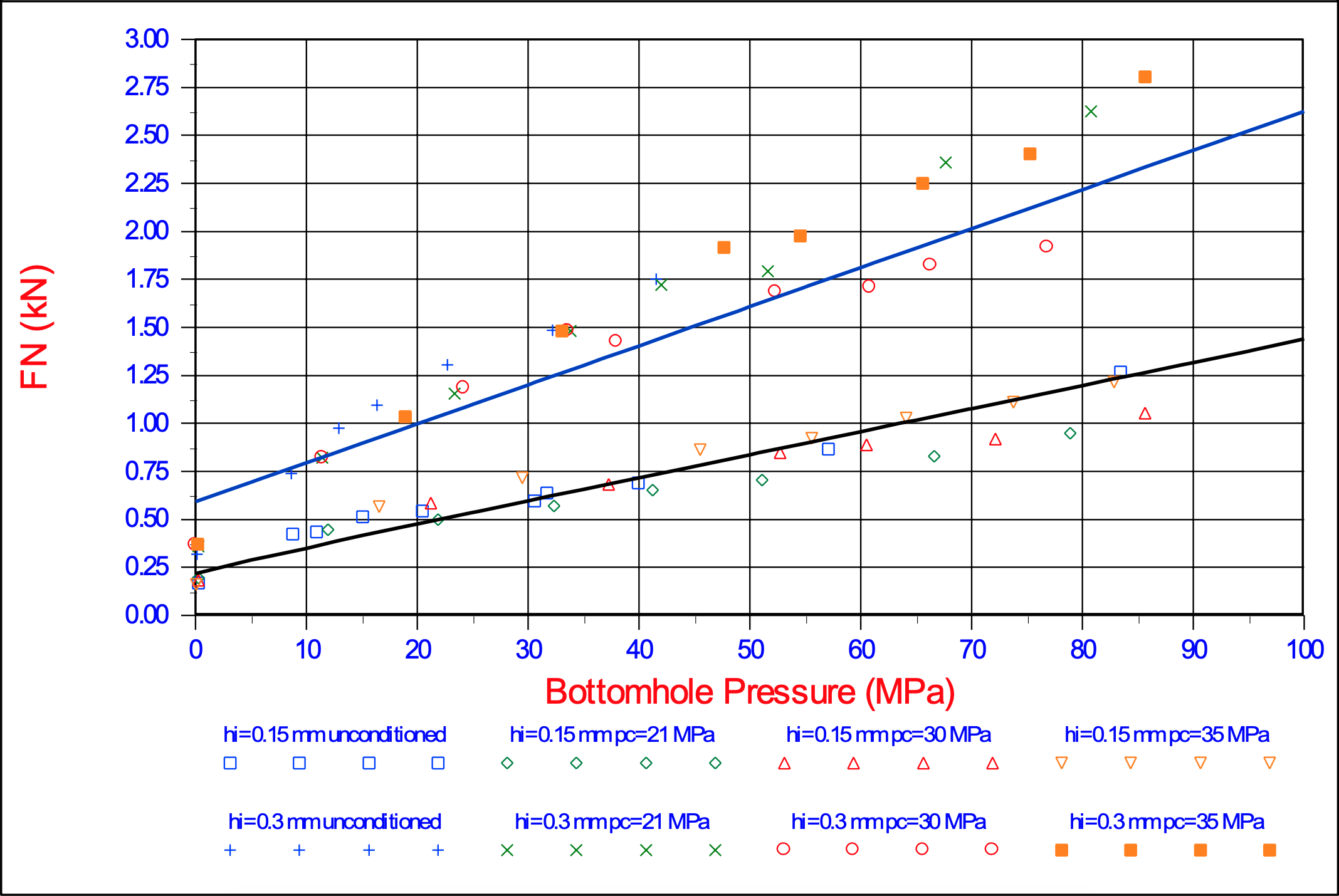
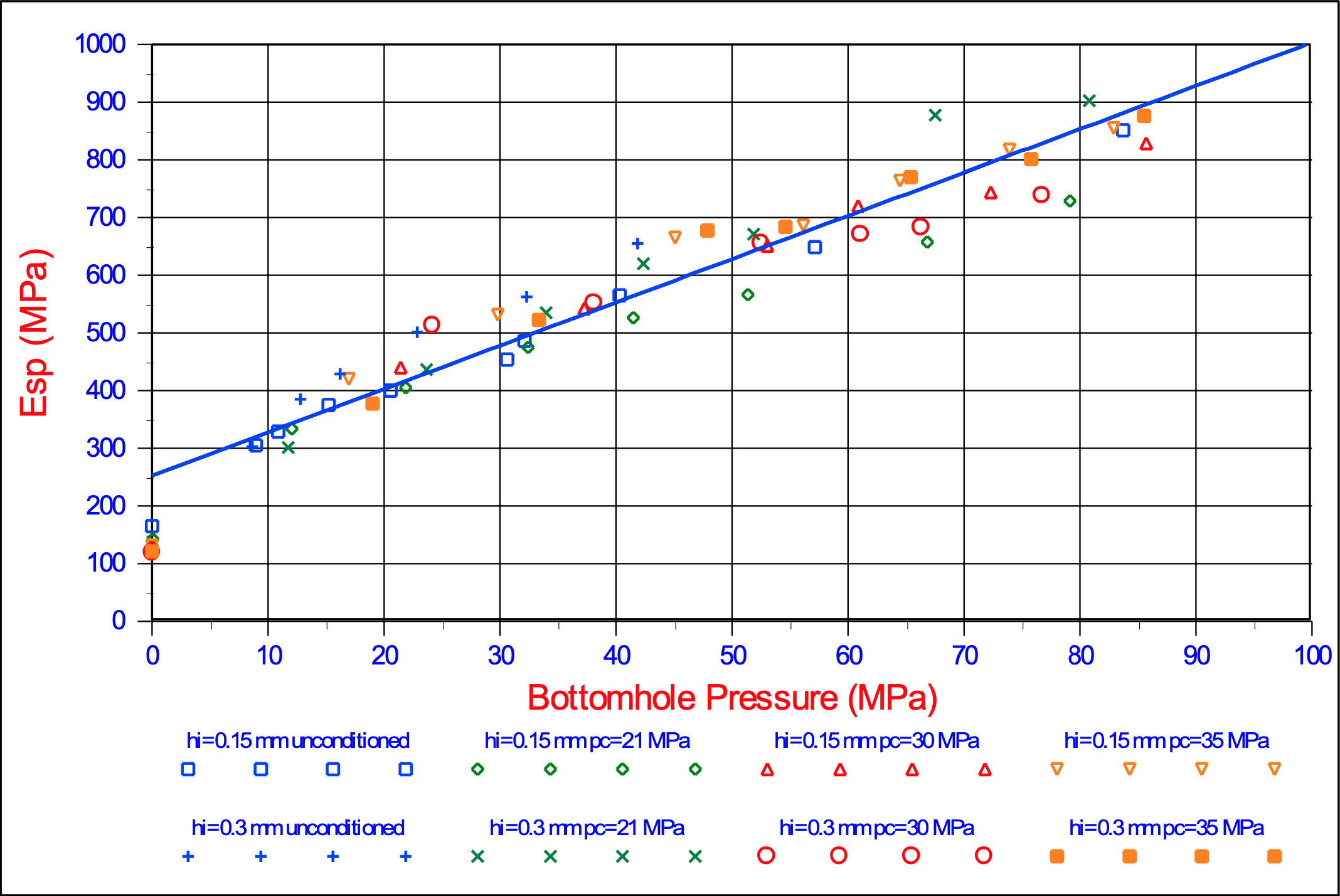
The theory developed here, which basically is the theory of Miedema (1987 September) extended with the Curling Type, has been applied on the cutting tests of Zijsling (1987). Zijsling conducted cutting tests with a PDC bit with a width and height of 10 mm in Mancos Shale. This type of rock has a UCS value of about 65 MPa, a cohesive shear strength c of about 25 MPa, an internal friction angle φ of 23o, according to Detournay & Atkinson (2000), a layer thickness hi of 0.15 mm and 0.30 mm and a blade angle α of 110o. The external friction angle δ is chosen at 2/3 of the internal friction angle φ. Based on the principle of minimum energy a shear angle β of 12o has been derived. Zijsling already concluded that balling would occur. Using equation (9-26) an effective blade height hb,m = 4.04·hi has been found. Figure 9-22 shows the cutting forces as measured by Zijsling compared with the theory derived here. The force FD is the force Fh in the direction of the cutting velocity and the force FN is the force Fv normal to the velocity direction. Figure 9-23 shows the specific energy Esp and the so called drilling strength S. Figure 9-29 and Figure 9-30 show the specific energy Esp as a function of the UCS value of a rock for different UCS/BTS ratio’s and different water depths. Figure 9-29 shows this for a 110o blade as in the experiments of Zijsling (1987). The UCS value of the Mancos Shale is about 65 MPa. It is clear that in this graph the UCS/BTS value has no influence, since there will be no tensile failure at a blade angle of 110o. There could however be brittle shear failure under atmospheric conditions resulting in a specific energy of 30%-50% of the lowest line in the graph. Figure 9-29 gives a good indication of the specific energy for drilling purposes.
Figure 9-30 and Figure 9-31 show this for a 45o and a 60o blade as may be used in dredging and mining. From this figure it is clear that under atmospheric conditions tensile failure may occur. The lines for the UCS/BTS ratios give the specific energy based on the peak forces. This specific energy should be multiplied with 30%-50% to get the average value. Roxborough (1987) found that for all sedimentary rocks and some sandstone, the specific energy is about 25% of the UCS value (both have the dimension kPa or MPa). In Figure 9-30 and Figure 9-31 this would match brittle-shear failure with a factor of 30%-50% (R=2). In dredging and mining the blade angle would normally be in a range of 45o to 60o. Vlasblom (2003-2007) uses a percentage of 40% of the UCS value for the specific energy based on the experience of the dredging industry, which is close to the value found by Roxborough (1987). The percentage used by Vlasblom has the purpose of production estimation and is on the safe side (a bit too high). Both the percentages of Roxborough (1987) and Vlasblom (2003-2007) are based on the brittle shear failure. In the case of brittle tensile failure the specific energy may be much lower.
Resuming it can be stated that the theory developed here matches the measurements of Zijsling (1987) well. It has been proven that the approach of Detournay & Atkinson (2000) misses the pore pressure force on the blade and thus leads to some wrong conclusions. It can further be stated that brittle tensile failure will only occur with relatively small blade angles under atmospheric conditions. Brittle shear failure may also occur with large blade angles under atmospheric conditions. The measurements of Zijsling show clearly that at 0 MPa bottom hole pressure, the average cutting forces are 30%-50% of the forces that would be expected based on the trend. The conclusions are valid for the experiments they are based on. In other types of rock or with other blade angles the theory may have to be adjusted. This can be taken into account by the following equation, where α will have a value of 3-7 depending on the type of material.
\[\ \mathrm{F_{h, c}=F_{h} \cdot\left(1-\frac{\alpha}{(z+10)}\right)}\tag{9-33}\]
At zero water depth the cutting forces are reduced to α/10, so to 30%-70% depending on the type of rock. At 90 m water depth the reduction is just 3%-7%, matching the Zijsling (1987) experiments, but also the Rafatian et al. (2009) and Kaitkay & Lei (2005) experiments. The equation is empirical and a first attempt, so it needs improvement.
Figure 9-24 and Figure 9-25 show the hb,m/hi ratio and the shear angle β. The Zijsling (1987) experiments match the curves of an internal friction angle of 25 degrees close. Since the blade height in these experiments was about 10 mm, the actual hb,m/hi ratio were 10/.15=66.66 and 10/.3=33.33. In both cases these ratios are much larger than the ones calculated for the Curling Type, leading to the conclusion that the Curling Type always occurs. So in offshore drilling, the Curling Type is the dominant cutting mechanism. On the horizontal axis, a value of 1 matches the shear strength of the rock, being about 25 MPa. A value of 4 matches the maximum hydrostatic pressure of 100 MPa as used in the experiments. The hb,m/hi ratio increases slightly with increasing hydrostatic pressure, the shear angle decreases slightly.
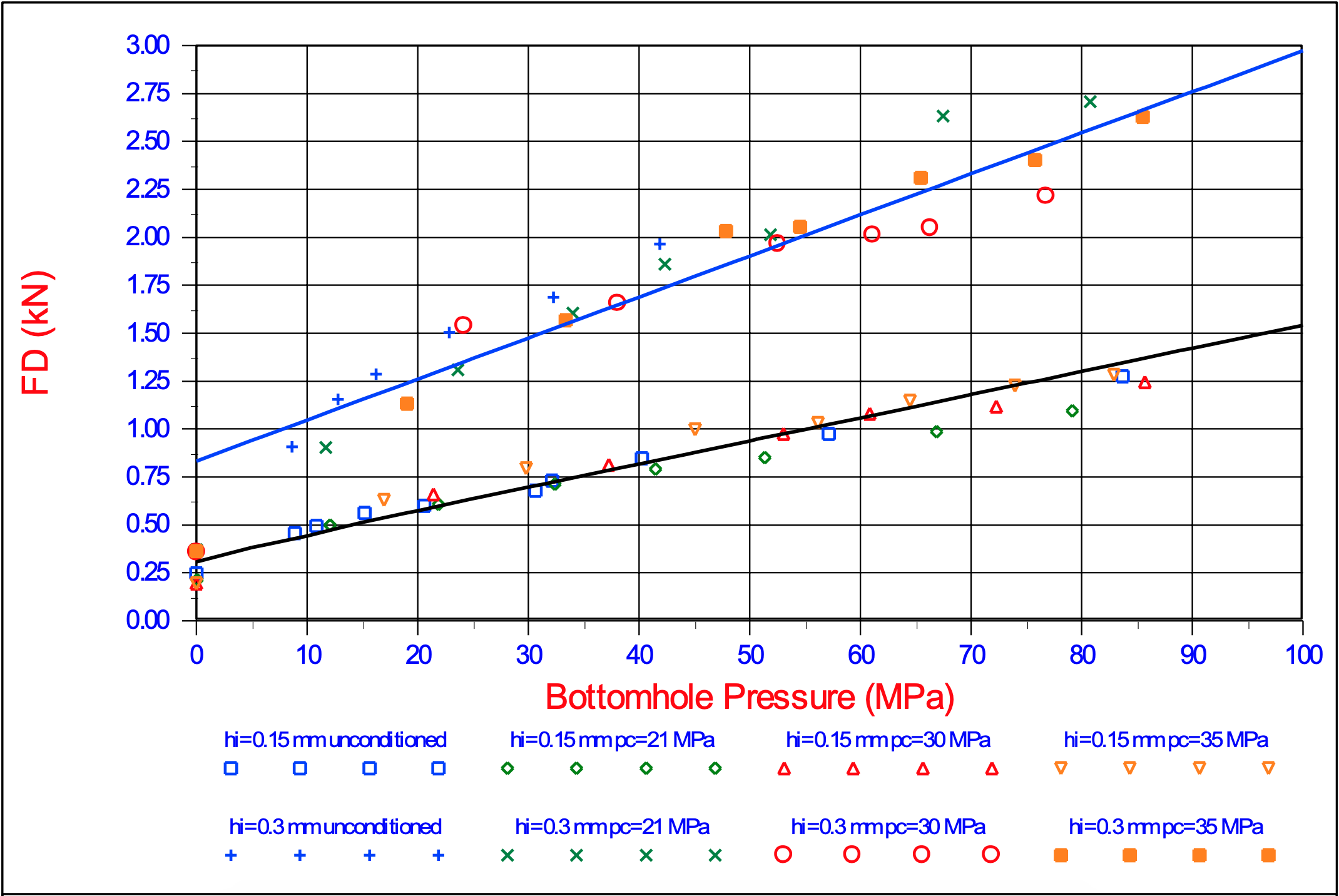
Blade angle α = 110o, blade width w = 10 mm, internal friction angle φ = 23.8o, external friction angle δ = 15.87o, shear strength c = 24.82 MPa, shear angle β = 12.00o, layer thickness hi = 0.15 mm and 0.30 mm, effective blade height hb = 4.04·hi.
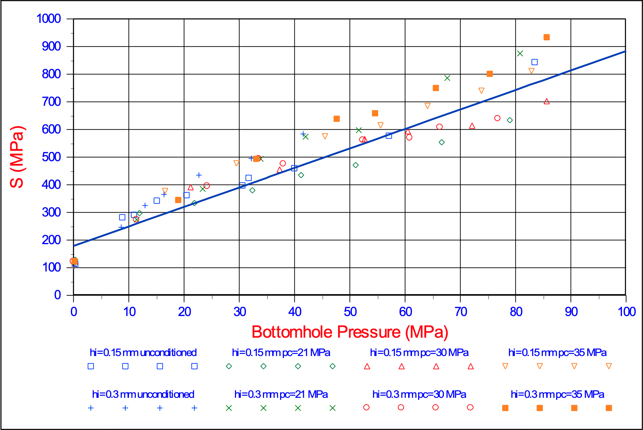
Blade angle α = 110o, blade width w = 10 mm, internal friction angle φ = 23.8o, external friction angle δ = 15.87o, shear strength c = 24.82 MPa, shear angle β = 12.00o, layer thickness hi = 0.15 mm and 0.30 mm, effective blade height hb = 4.04·hi.
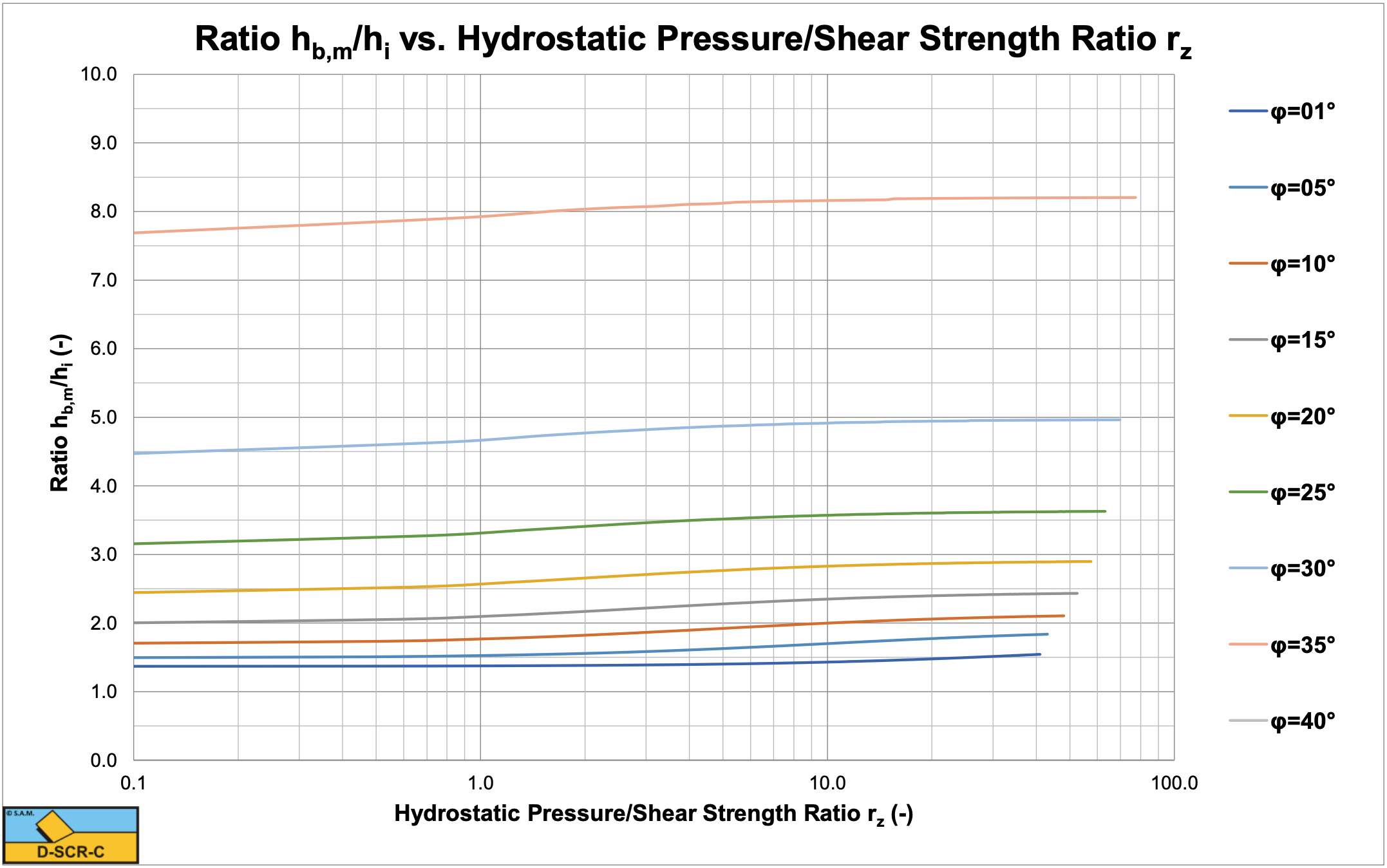
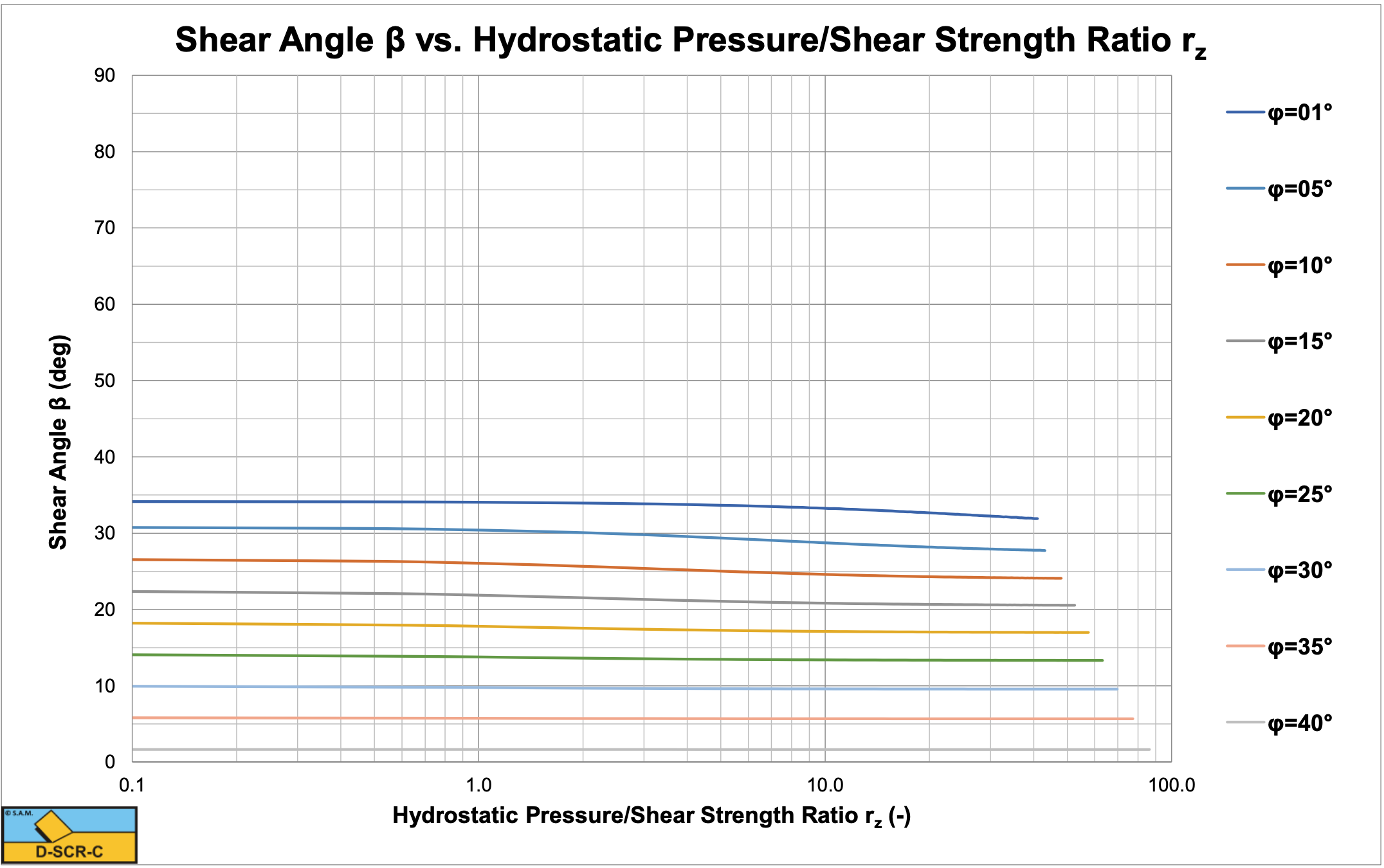
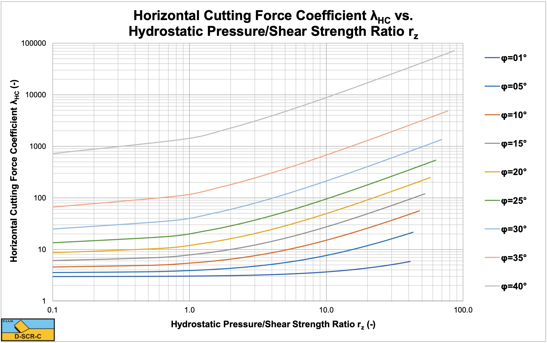
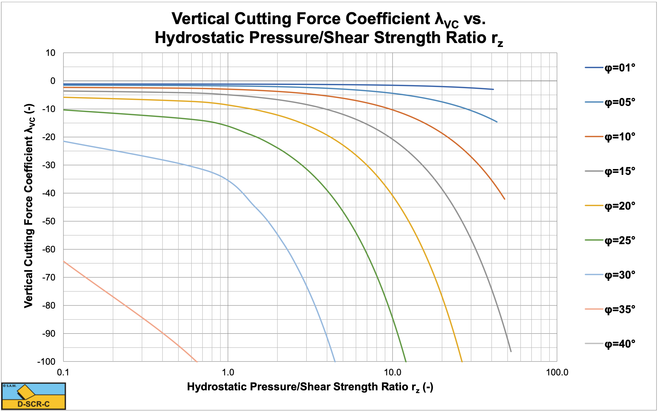
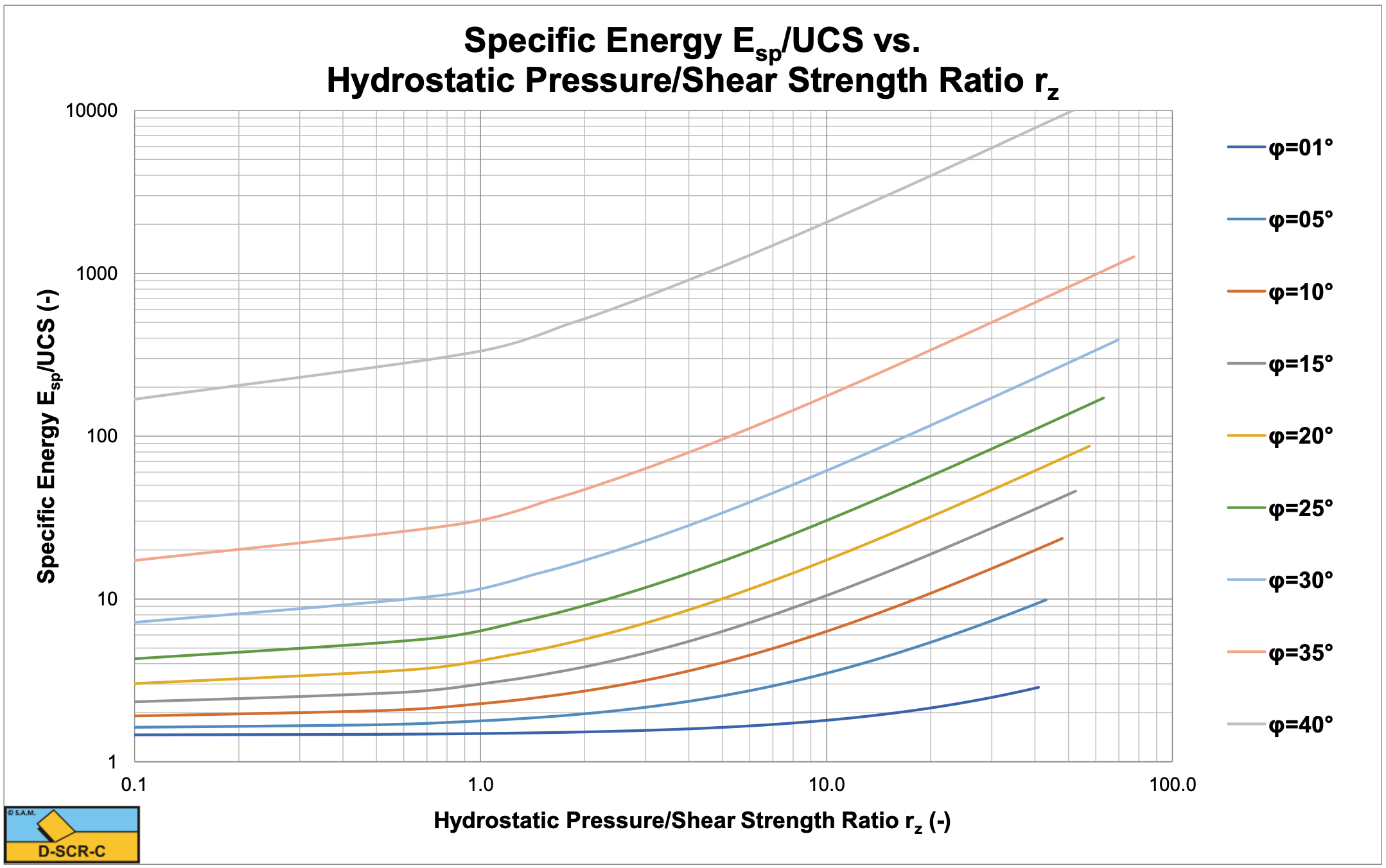
Figure 9-26 and Figure 9-27 show the horizontal and vertical cutting force coefficients. For a hydrostatic pressure of 100 MPa and an internal friction angle of 25 degrees the graphs give a horizontal cutting force coefficient of λHC=45 and a vertical cutting force coefficient of λVC=38 giving cutting forces of Fh=FD=3.25 kN and Fv=FN=2.74 kN, matching the experiments in Figure 9-22. Figure 9-28 shows the Esp/UCS ratio, which is very convenient for production estimation.