3.1: The cross-entropy cost function

When a golf player is first learning to play golf, they usually spend most of their time developing a basic swing. Only gradually do they develop other shots, learning to chip, draw and fade the ball, building on and modifying their basic swing. In a similar way, up to now we've focused on understanding the backpropagation algorithm. It's our "basic swing", the foundation for learning in most work on neural networks. In this chapter I explain a suite of techniques which can be used to improve on our vanilla implementation of backpropagation, and so improve the way our networks learn.

The techniques we'll develop in this chapter include: a better choice of cost function, known as the cross-entropy cost function; four so-called "regularization" methods (L1 and L2 regularization, dropout, and artificial expansion of the training data), which make our networks better at generalizing beyond the training data; a better method for initializing the weights in the network; and a set of heuristics to help choose good hyper-parameters for the network. I'll also overview several other techniques in less depth. The discussions are largely independent of one another, and so you may jump ahead if you wish. We'll also implement many of the techniques in running code, and use them to improve the results obtained on the handwriting classification problem studied in Chapter 1.

Of course, we're only covering a few of the many, many techniques which have been developed for use in neural nets. The philosophy is that the best entree to the plethora of available techniques is in-depth study of a few of the most important. Mastering those important techniques is not just useful in its own right, but will also deepen your understanding of what problems can arise when you use neural networks. That will leave you well prepared to quickly pick up other techniques, as you need them.

The cross-entropy cost function

Most of us find it unpleasant to be wrong. Soon after beginning to learn the piano I gave my first performance before an audience. I was nervous, and began playing the piece an octave too low. I got confused, and couldn't continue until someone pointed out my error. I was very embarrassed. Yet while unpleasant, we also learn quickly when we're decisively wrong. You can bet that the next time I played before an audience I played in the correct octave! By contrast, we learn more slowly when our errors are less well-defined.

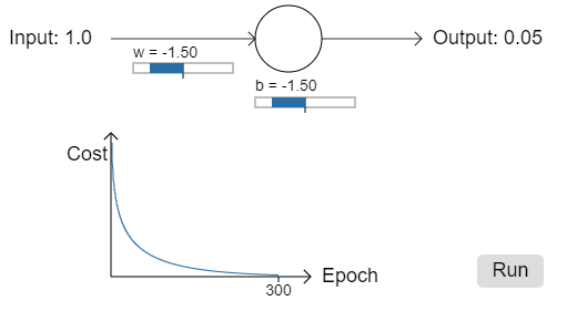
Ideally, we hope and expect that our neural networks will learn fast from their errors. Is this what happens in practice? To answer this question, let's look at a toy example. The example involves a neuron with just one input:

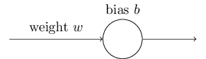
We'll train this neuron to do something ridiculously easy: take the input 1 to the output 0. Of course, this is such a trivial task that we could easily figure out an appropriate weight and bias by hand, without using a learning algorithm. However, it turns out to be illuminating to use gradient descent to attempt to learn a weight and bias. So let's take a look at how the neuron learns.

To make things definite, I'll pick the initial weight to be 0.6 and the initial bias to be 0.9. These are generic choices used as a place to begin learning, I wasn't picking them to be special in any way. The initial output from the neuron is 0.820.82, so quite a bit of learning will be needed before our neuron gets near the desired output, 0.0. Click on "Run" in the bottom right corner below to see how the neuron learns an output much closer to 0.0. Note that this isn't a pre-recorded animation, your browser is actually computing the gradient, then using the gradient to update the weight and bias, and displaying the result. The learning rate is \(η=0.15\), which turns out to be slow enough that we can follow what's happening, but fast enough that we can get substantial learning in just a few seconds. The cost is the quadratic cost function, \(C\), introduced back in Chapter 1. I'll remind you of the exact form of the cost function shortly, so there's no need to go and dig up the definition. Note that you can run the animation multiple times by clicking on "Run" again.

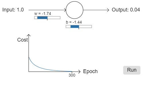
As you can see, the neuron rapidly learns a weight and bias that drives down the cost, and gives an output from the neuron of about 0.09. That's not quite the desired output, 0.0, but it is pretty good. Suppose, however, that we instead choose both the starting weight and the starting bias to be 2.0. In this case the initial output is 0.98, which is very badly wrong. Let's look at how the neuron learns to output 0 in this case. Click on "Run" again:

Although this example uses the same learning rate (η=0.15), we can see that learning starts out much more slowly. Indeed, for the first 150 or so learning epochs, the weights and biases don't change much at all. Then the learning kicks in and, much as in our first example, the neuron's output rapidly moves closer to 0.0.

This behaviour is strange when contrasted to human learning. As I said at the beginning of this section, we often learn fastest when we're badly wrong about something. But we've just seen that our artificial neuron has a lot of difficulty learning when it's badly wrong - far more difficulty than when it's just a little wrong. What's more, it turns out that this behaviour occurs not just in this toy model, but in more general networks. Why is learning so slow? And can we find a way of avoiding this slowdown?

To understand the origin of the problem, consider that our neuron learns by changing the weight and bias at a rate determined by the partial derivatives of the cost function, \(∂C/∂w\) and \(∂C/∂b\). So saying "learning is slow" is really the same as saying that those partial derivatives are small. The challenge is to understand why they are small. To understand that, let's compute the partial derivatives. Recall that we're using the quadratic cost function, which, from Equation (6), is given by

\[ C=\frac{(y−a)^2}{2},\label{54}\tag{54} \]

where a is the neuron's output when the training input \(x=1\) is used, and \(y=0\) is the corresponding desired output. To write this more explicitly in terms of the weight and bias, recall that \(a=σ(z)\), where \(z=wx+b\). Using the chain rule to differentiate with respect to the weight and bias we get

\[ \frac{∂C}{∂w}=(a−y)σ′(z)x=aσ′(z)\label{55}\tag{55} \]

\[ \frac{∂C}{∂w}=(a−y)σ′(z)=aσ′(z)\label{56}\tag{56} \]

where I have substituted \(x=1\) and \(y=0\). To understand the behaviour of these expressions, let's look more closely at the \(σ′(z)\) term on the right-hand side. Recall the shape of the \(σ\) function:

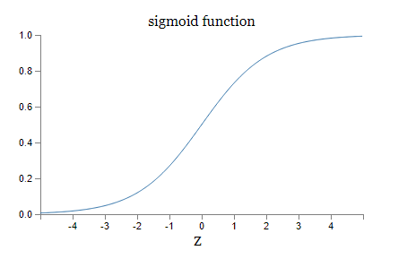
We can see from this graph that when the neuron's output is close to 1, the curve gets very flat, and so \(σ′(z)\) gets very small. Equations \ref{55} and \ref{56} then tell us that \(∂C/∂w\) and \(∂C/∂b\) get very small. This is the origin of the learning slowdown. What's more, as we shall see a little later, the learning slowdown occurs for essentially the same reason in more general neural networks, not just the toy example we've been playing with.

Introducing the cross-entropy cost function

How can we address the learning slowdown? It turns out that we can solve the problem by replacing the quadratic cost with a different cost function, known as the cross-entropy. To understand the cross-entropy, let's move a little away from our super-simple toy model. We'll suppose instead that we're trying to train a neuron with several input variables, \(x1,x2,…\), corresponding weights \(w1,w2,…\), and a bias, b:

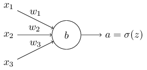
The output from the neuron is, of course, \(a=σ(z)\), where \(z=\sum_j{w_jx_j+b}\) is the weighted sum of the inputs. We define the cross-entropy cost function for this neuron by

\[ C=−\frac{1}{n}\sum_x{[ylna+(1−y)ln(1−a)]},\label{57}\tag{57} \]

where n is the total number of items of training data, the sum is over all training inputs, \(x\), and \(y\) is the corresponding desired output.

It's not obvious that the expression \(\ref{57}\) fixes the learning slowdown problem. In fact, frankly, it's not even obvious that it makes sense to call this a cost function! Before addressing the learning slowdown, let's see in what sense the cross-entropy can be interpreted as a cost function.

Two properties in particular make it reasonable to interpret the cross-entropy as a cost function. First, it's non-negative, that is, \(C>0\). To see this, notice that: (a) all the individual terms in the sum in \(\ref{57}\) are negative, since both logarithms are of numbers in the range 0 to 1; and (b) there is a minus sign out the front of the sum.

Second, if the neuron's actual output is close to the desired output for all training inputs, \(x\), then the cross-entropy will be close to zero*

*To prove this I will need to assume that the desired outputs \(y\) are all either 0 or 1. This is usually the case when solving classification problems, for example, or when computing Boolean functions. To understand what happens when we don't make this assumption, see the exercises at the end of this section. To see this, suppose for example that \(y=0\) and \(a≈0\) for some input \(x\). This is a case when the neuron is doing a good job on that input. We see that the first term in the expression \ref{57} for the cost vanishes, since \(y=0\), while the second term is just \(−ln(1−a)≈0\). A similar analysis holds when \(y=1\) and \(a≈1\). And so the contribution to the cost will be low provided the actual output is close to the desired output.

Summing up, the cross-entropy is positive, and tends toward zero as the neuron gets better at computing the desired output, \(y\), for all training inputs, \(x\). These are both properties we'd intuitively expect for a cost function. Indeed, both properties are also satisfied by the quadratic cost. So that's good news for the cross-entropy. But the cross-entropy cost function has the benefit that, unlike the quadratic cost, it avoids the problem of learning slowing down. To see this, let's compute the partial derivative of the cross-entropy cost with respect to the weights. We substitute \(a=σ(z)\) into \ref{57}, and apply the chain rule twice, obtaining:

\[ \begin{align} \frac{∂C}{∂w_j} & =−\frac{1}{n}\sum_x{\left(\frac{y}{σ(z)}−\frac{(1−y)}{1−σ(z)}\right)\frac{∂σ}{∂w_j}}\label{58}\tag{58} \\ & =−\frac{1}{n}\sum_x{\left(\frac{y}{σ(z)}−\frac{(1−y)}{1−σ(z)}\right)σ′(z)x_j}\label{59}\tag{59} \end{align} \]

Putting everything over a common denominator and simplifying this becomes:

\[ \frac{∂C}{∂w_j} =\frac{1}{n}\sum_x{\frac{σ′(z)x_j}{σ(z)(1−σ(z))}(σ(z)−y)}.\label{60}\tag{60} \]

Using the definition of the sigmoid function, \(σ(z)=1/(1+e^{−z})\), and a little algebra we can show that \(σ′(z)=σ(z)(1−σ(z))\). I'll ask you to verify this in an exercise below, but for now let's accept it as given. We see that the \(σ′(z)\) and \(σ(z)(1−σ(z))\) terms cancel in the equation just above, and it simplifies to become:

\[ \frac{∂C}{∂w_j} = \frac{1}{n}\sum_x{x_j(σ(z)−y)}.\label{61}\tag{61} \]

This is a beautiful expression. It tells us that the rate at which the weight learns is controlled by \(σ(z)−y\), i.e., by the error in the output. The larger the error, the faster the neuron will learn. This is just what we'd intuitively expect. In particular, it avoids the learning slowdown caused by the \(σ′(z)\) term in the analogous equation for the quadratic cost, Equation \(\ref{55}\). When we use the cross-entropy, the \(σ′(z)\) term gets canceled out, and we no longer need worry about it being small. This cancellation is the special miracle ensured by the cross-entropy cost function. Actually, it's not really a miracle. As we'll see later, the cross-entropy was specially chosen to have just this property.

In a similar way, we can compute the partial derivative for the bias. I won't go through all the details again, but you can easily verify that

\[ \frac{∂C}{∂b} =\frac{1}{n}\sum_x{(σ(z)−y)}.\label{62}\tag{62} \]

Again, this avoids the learning slowdown caused by the \(σ′(z)\) term in the analogous equation for the quadratic cost, Equation \(\ref{56}\).

Exercise

• Verify that \(σ′(z)=σ(z)(1−σ(z)).\)

Let's return to the toy example we played with earlier, and explore what happens when we use the cross-entropy instead of the quadratic cost. To re-orient ourselves, we'll begin with the case where the quadratic cost did just fine, with starting weight 0.6 and starting bias 0.9. Press "Run" to see what happens when we replace the quadratic cost by the cross-entropy:

Unsurprisingly, the neuron learns perfectly well in this instance, just as it did earlier. And now let's look at the case where our neuron got stuck before (link, for comparison), with the weight and bias both starting at 2.0:

Success! This time the neuron learned quickly, just as we hoped. If you observe closely you can see that the slope of the cost curve was much steeper initially than the initial flat region on the corresponding curve for the quadratic cost. It's that steepness which the cross-entropy buys us, preventing us from getting stuck just when we'd expect our neuron to learn fastest, i.e., when the neuron starts out badly wrong.

I didn't say what learning rate was used in the examples just illustrated. Earlier, with the quadratic cost, we used \(η=0.15\). Should we have used the same learning rate in the new examples? In fact, with the change in cost function it's not possible to say precisely what it means to use the "same" learning rate; it's an apples and oranges comparison. For both cost functions I simply experimented to find a learning rate that made it possible to see what is going on. If you're still curious, despite my disavowal, here's the lowdown: I used \(η=0.005\) in the examples just given.

You might object that the change in learning rate makes the graphs above meaningless. Who cares how fast the neuron learns, when our choice of learning rate was arbitrary to begin with?! That objection misses the point. The point of the graphs isn't about the absolute speed of learning. It's about how the speed of learning changes. In particular, when we use the quadratic cost learning is slower when the neuron is unambiguously wrong than it is later on, as the neuron gets closer to the correct output; while with the cross-entropy learning is faster when the neuron is unambiguously wrong. Those statements don't depend on how the learning rate is set.

We've been studying the cross-entropy for a single neuron. However, it's easy to generalize the cross-entropy to many-neuron multi-layer networks. In particular, suppose \(y=y1,y2,…\) are the desired values at the output neurons, i.e., the neurons in the final layer, while \(a^L_1,a^L_2,…\) are the actual output values. Then we define the cross-entropy by

\[ C=−\frac{1}{n}\sum_x{}\sum_j{\left[y_jlna^L_j+(1−y_j)ln(1−a^L_j)\right]}.\label{63}\tag{63} \]

This is the same as our earlier expression, Equation \(\ref{57}\), except now we've got the \(\sum_j{}\) summing over all the output neurons. I won't explicitly work through a derivation, but it should be plausible that using the expression \(\ref{63}\) avoids a learning slowdown in many-neuron networks. If you're interested, you can work through the derivation in the problem below.

Incidentally, I'm using the term "cross-entropy" in a way that has confused some early readers, since it superficially appears to conflict with other sources. In particular, it's common to define the cross-entropy for two probability distributions, \(p_j\) and \(q_j\), as \(\sum_j{p_jlnq_j}\). This definition may be connected to \(ref{57}\), if we treat a single sigmoid neuron as outputting a probability distribution consisting of the neuron's activation aa and its complement \(1−a\).

However, when we have many sigmoid neurons in the final layer, the vector \(a^L_j\) of activations don't usually form a probability distribution. As a result, a definition like \(\sum_j{p_jlnq_j}\) doesn't even make sense, since we're not working with probability distributions. Instead, you can think of \ref{63} as a summed set of per-neuron cross-entropies, with the activation of each neuron being interpreted as part of a two-element probability distribution*. In this sense, \ref{63} is a generalization of the cross-entropy for probability distributions.

*Of course, in our networks there are no probabilistic elements, so they're not really probabilities.

When should we use the cross-entropy instead of the quadratic cost? In fact, the cross-entropy is nearly always the better choice, provided the output neurons are sigmoid neurons. To see why, consider that when we're setting up the network we usually initialize the weights and biases using some sort of randomization. It may happen that those initial choices result in the network being decisively wrong for some training input - that is, an output neuron will have saturated near 1, when it should be 0, or vice versa. If we're using the quadratic cost that will slow down learning. It won't stop learning completely, since the weights will continue learning from other training inputs, but it's obviously undesirable.

Exercises

• One gotcha with the cross-entropy is that it can be difficult at first to remember the respective roles of the \(ys\) and the \(as\). It's easy to get confused about whether the right form is \(−[ylna+(1−y)ln(1−a)]\) or \(−[alny+(1−a)ln(1−y)]\).What happens to the second of these expressions when \(y=0\) or 1? Does this problem afflict the first expression? Why or why not?
• In the single-neuron discussion at the start of this section, I argued that the cross-entropy is small if \(σ(z)≈y\) for all training inputs. The argument relied on \(y\) being equal to either 0 or 1. This is usually true in classification problems, but for other problems (e.g., regression problems) y can sometimes take values intermediate between 0 and 1. Show that the cross-entropy is still minimized when \(σ(z)=y\) for all training inputs. When this is the case the cross-entropy has the value:

  \[ C=−\frac{1}{n}\sum_x{[ylny+(1−y)ln(1−y)]}.\label{64}\tag{64} \]

  The quantity \(−[ylny+(1−y)ln(1−y)]\) is sometimes known as the binary entropy.

Problems

• Many-layer multi-neuron networks In the notation introduced in the last chapter, show that for the quadratic cost the partial derivative with respect to weights in the output layer is

  \[ \frac{∂C}{∂w^L_{jk}} = \frac{1}{n}\sum_x{a^{L−1}_k(a^L_j−y_j)σ′(z^L_j)}.\label{65}\tag{65} \]

  The term \(σ′(z^L_j)\) causes a learning slowdown whenever an output neuron saturates on the wrong value. Show that for the cross-entropy cost the output error \(δ^L\) for a single training example \(x\) is given by

  \[ δ^L=a^L−y.\label{66}\tag{66} \]

  Use this expression to show that the partial derivative with respect to the weights in the output layer is given by

  \[ \frac{∂C}{∂w^L_{jk}} = \frac{1}{n}\sum_x{a^{L−1}_k(a^L_j−yj)}.\label{67}\tag{67} \]

  The \(σ′(z^L_j)\) term has vanished, and so the cross-entropy avoids the problem of learning slowdown, not just when used with a single neuron, as we saw earlier, but also in many-layer multi-neuron networks. A simple variation on this analysis holds also for the biases. If this is not obvious to you, then you should work through that analysis as well.
• Using the quadratic cost when we have linear neurons in the output layer Suppose that we have a many-layer multi-neuron network. Suppose all the neurons in the final layer are linear neurons, meaning that the sigmoid activation function is not applied, and the outputs are simply \(a^L_j=z^L_j\). Show that if we use the quadratic cost function then the output error \(δ^L\) for a single training example \(x\) is given by

  \[ δ^L=a^L−y.\label{68}\tag{68} \]

  Similarly to the previous problem, use this expression to show that the partial derivatives with respect to the weights and biases in the output layer are given by

  \[ \frac{∂C}{∂w^L_{jk}} =\frac{1}{n}\sum_x{a^{L−1}_k(a^L_j−y_j)}.\label{69}\tag{69} \]

$$ \frac{∂C}{∂b^L_j} = \frac{1}{n}\sum_x{(a^L_j−y_j).}\label{70}\tag{70} \]

This shows that if the output neurons are linear neurons then the quadratic cost will not give rise to any problems with a learning slowdown. In this case the quadratic cost is, in fact, an appropriate cost function to use.

Using the cross-entropy to classify MNIST digits

The cross-entropy is easy to implement as part of a program which learns using gradient descent and backpropagation. We'll do that later in the chapter, developing an improved version of our earlier program for classifying the MNIST handwritten digits, network.py. The new program is called network2.py, and incorporates not just the cross-entropy, but also several other techniques developed in this chapter*

*The code is available on GitHub.

For now, let's look at how well our new program classifies MNIST digits. As was the case in Chapter 1, we'll use a network with \(30\) hidden neurons, and we'll use a mini-batch size of \(10\). We set the learning rate to \(η=0.5\)*and we train for \(30\) epochs. The interface to network2.py is slightly different than network.py, but it should still be clear what is going on. You can, by the way, get documentation about network2.py's interface by using commands such as help(network2.Network.SGD) in a Python shell.

*In Chapter 1 we used the quadratic cost and a learning rate of \(η=3.0\). As discussed above, it's not possible to say precisely what it means to use the "same" learning rate when the cost function is changed. For both cost functions I experimented to find a learning rate that provides near-optimal performance, given the other hyper-parameter choices.

There is, incidentally, a very rough general heuristic for relating the learning rate for the cross-entropy and the quadratic cost. As we saw earlier, the gradient terms for the quadratic cost have an extra \(σ′=σ(1−σ)\) term in them. Suppose we average this over values for \(σ\), \(\int_0^1 dσσ(1−σ)=1/6\). We see that (very roughly) the quadratic cost learns an average of \(6\) times slower, for the same learning rate. This suggests that a reasonable starting point is to divide the learning rate for the quadratic cost by \(6\). Of course, this argument is far from rigorous, and shouldn't be taken too seriously. Still, it can sometimes be a useful starting point.

>>> import mnist_loader
>>> training_data, validation_data, test_data = \
... mnist_loader.load_data_wrapper()
>>> import network2
>>> net = network2.Network([784, 30, 10], cost=network2.CrossEntropyCost)
>>> net.large_weight_initializer()
>>> net.SGD(training_data, 30, 10, 0.5, evaluation_data=test_data,
... monitor_evaluation_accuracy=True)

Note, by the way, that the net.large_weight_initializer() command is used to initialize the weights and biases in the same way as described in Chapter 1. We need to run this command because later in this chapter we'll change the default weight initialization in our networks. The result from running the above sequence of commands is a network with \(95.49\) percent accuracy. This is pretty close to the result we obtained in Chapter 1, \(95.42\) percent, using the quadratic cost.

Let's look also at the case where we use \(100\) hidden neurons, the cross-entropy, and otherwise keep the parameters the same. In this case we obtain an accuracy of \(96.82\) percent. That's a substantial improvement over the results from Chapter 1, where we obtained a classification accuracy of \(96.59\) percent, using the quadratic cost. That may look like a small change, but consider that the error rate has dropped from \(3.41\) percent to \(3.18\) percent. That is, we've eliminated about one in fourteen of the original errors. That's quite a handy improvement.

It's encouraging that the cross-entropy cost gives us similar or better results than the quadratic cost. However, these results don't conclusively prove that the cross-entropy is a better choice. The reason is that I've put only a little effort into choosing hyper-parameters such as learning rate, mini-batch size, and so on. For the improvement to be really convincing we'd need to do a thorough job optimizing such hyper-parameters. Still, the results are encouraging, and reinforce our earlier theoretical argument that the cross-entropy is a better choice than the quadratic cost.

This, by the way, is part of a general pattern that we'll see through this chapter and, indeed, through much of the rest of the book. We'll develop a new technique, we'll try it out, and we'll get "improved" results. It is, of course, nice that we see such improvements. But the interpretation of such improvements is always problematic. They're only truly convincing if we see an improvement after putting tremendous effort into optimizing all the other hyper-parameters. That's a great deal of work, requiring lots of computing power, and we're not usually going to do such an exhaustive investigation. Instead, we'll proceed on the basis of informal tests like those done above. Still, you should keep in mind that such tests fall short of definitive proof, and remain alert to signs that the arguments are breaking down.

By now, we've discussed the cross-entropy at great length. Why go to so much effort when it gives only a small improvement to our MNIST results? Later in the chapter we'll see other techniques - notably, regularization - which give much bigger improvements. So why so much focus on cross-entropy? Part of the reason is that the cross-entropy is a widely-used cost function, and so is worth understanding well. But the more important reason is that neuron saturation is an important problem in neural nets, a problem we'll return to repeatedly throughout the book. And so I've discussed the cross-entropy at length because it's a good laboratory to begin understanding neuron saturation and how it may be addressed.

What does the cross-entropy mean? Where does it come from?

Our discussion of the cross-entropy has focused on algebraic analysis and practical implementation. That's useful, but it leaves unanswered broader conceptual questions, like: what does the cross-entropy mean? Is there some intuitive way of thinking about the cross-entropy? And how could we have dreamed up the cross-entropy in the first place?

Let's begin with the last of these questions: what could have motivated us to think up the cross-entropy in the first place? Suppose we'd discovered the learning slowdown described earlier, and understood that the origin was the \(σ′(z)\) terms in Equations \(\ref{55}\) and \(\ref{56}\). After staring at those equations for a bit, we might wonder if it's possible to choose a cost function so that the \(σ′(z)\) term disappeared. In that case, the cost \(C=C_x\) for a single training example \(x\) would satisfy

\[ \frac{∂C}{∂w_j} = x_j(a−y)\label{71}\tag{71} \]

\[ \frac{∂C}{∂b} = (a−y).\label{72}\tag{72} \]

If we could choose the cost function to make these equations true, then they would capture in a simple way the intuition that the greater the initial error, the faster the neuron learns. They'd also eliminate the problem of a learning slowdown. In fact, starting from these equations we'll now show that it's possible to derive the form of the cross-entropy, simply by following our mathematical noses. To see this, note that from the chain rule we have

\[ \frac{∂C}{∂b} = \frac{∂C}{∂a}σ′(z).\label{73}\tag{73} \]

Using \(σ′(z)=σ(z)(1−σ(z))=a(1−a)\) the last equation becomes

\[ \frac{∂C}{∂b} = \frac{∂C}{∂a}a(1−a).\label{74}\tag{74} \]

Comparing to Equation \(\ref{72}\) we obtain

\[ \frac{∂C}{∂a} = \frac{a−y}{a(1−a)}.\label{75}\tag{75} \]

Integrating this expression with respect to aa gives

\[ C=−[ylna+(1−y)ln(1−a)]+constant,\label{76}\tag{76} \]

for some constant of integration. This is the contribution to the cost from a single training example, \(x\). To get the full cost function we must average over training examples, obtaining

\[ C=−\frac{1}{n}\sum_x{[ylna+(1−y)ln(1−a)]}+constant,\label{77}\tag{77} \]

where the constant here is the average of the individual constants for each training example. And so we see that Equations \(\ref{71}\) and \(\ref{72}\) uniquely determine the form of the cross-entropy, up to an overall constant term. The cross-entropy isn't something that was miraculously pulled out of thin air. Rather, it's something that we could have discovered in a simple and natural way.

What about the intuitive meaning of the cross-entropy? How should we think about it? Explaining this in depth would take us further afield than I want to go. However, it is worth mentioning that there is a standard way of interpreting the cross-entropy that comes from the field of information theory. Roughly speaking, the idea is that the cross-entropy is a measure of surprise. In particular, our neuron is trying to compute the function \(x→y=y(x)\). But instead it computes the function \(x→a=a(x)\). Suppose we think of aa as our neuron's estimated probability that \(y\) is \(1\), and \(1−a\) is the estimated probability that the right value for \(y\) is \(0\). Then the cross-entropy measures how "surprised" we are, on average, when we learn the true value for \(y\). We get low surprise if the output is what we expect, and high surprise if the output is unexpected. Of course, I haven't said exactly what "surprise" means, and so this perhaps seems like empty verbiage. But in fact there is a precise information-theoretic way of saying what is meant by surprise. Unfortunately, I don't know of a good, short, self-contained discussion of this subject that's available online. But if you want to dig deeper, then Wikipedia contains a brief summary that will get you started down the right track. And the details can be filled in by working through the materials about the Kraft inequality in chapter 5 of the book about information theory by Cover and Thomas.

Problem

• We've discussed at length the learning slowdown that can occur when output neurons saturate, in networks using the quadratic cost to train. Another factor that may inhibit learning is the presence of the \(x_j\) term in Equation \(\ref{61}\). Because of this term, when an input \(x_j\) is near to zero, the corresponding weight \(w_j\) will learn slowly. Explain why it is not possible to eliminate the \(x_j\) term through a clever choice of cost function.

Softmax

In this chapter we'll mostly use the cross-entropy cost to address the problem of learning slowdown. However, I want to briefly describe another approach to the problem, based on what are called softmax layers of neurons. We're not actually going to use softmax layers in the remainder of the chapter, so if you're in a great hurry, you can skip to the next section. However, softmax is still worth understanding, in part because it's intrinsically interesting, and in part because we'll use softmax layers in Chapter 6, in our discussion of deep neural networks.

The idea of softmax is to define a new type of output layer for our neural networks. It begins in the same way as with a sigmoid layer, by forming the weighted inputs* \(z^L_j =\sum_k{w^L_{jk}a^{L−1}_k+b^L_j}.\)

*In describing the softmax we'll make frequent use of notation introduced in the last chapter. You may wish to revisit that chapter if you need to refresh your memory about the meaning of the notation.

However, we don't apply the sigmoid function to get the output. Instead, in a softmax layer we apply the so-called softmax function to the \(z^L_j\). According to this function, the activation \(a^L_j\) of the \(j^{th}\) output neuron is

\[ a^L_j = \frac{e^{z^L_j}}{\sum_x{e^{z^L_j}}},\label{78}\tag{78} \]

where in the denominator we sum over all the output neurons.

If you're not familiar with the softmax function, Equation \(\ref{78}\) may look pretty opaque. It's certainly not obvious why we'd want to use this function. And it's also not obvious that this will help us address the learning slowdown problem. To better understand Equation \(\ref{78}\), suppose we have a network with four output neurons, and four corresponding weighted inputs, which we'll denote \(z^L_1,z^L_2,z^L_3\), and \(z^L_4\). Shown below are adjustable sliders showing possible values for the weighted inputs, and a graph of the corresponding output activations. A good place to start exploration is by using the bottom slider to increase \(z^L_4\):

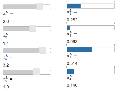
As you increase \(z^L_4\), you'll see an increase in the corresponding output activation, \(a^L_4\), and a decrease in the other output activations. Similarly, if you decrease \(z^L_4\) then \(a^L_4\) will decrease, and all the other output activations will increase. In fact, if you look closely, you'll see that in both cases the total change in the other activations exactly compensates for the change in \(a^L_4\). The reason is that the output activations are guaranteed to always sum up to \(1\), as we can prove using Equation \(\ref{78}\) and a little algebra:

\[ \sum_j{a^L_j} = \frac{\sum_j{e^{z^L_j}}}{\sum_k{e^{z^L_j}}} = 1.\label{79}\tag{79} \]

As a result, if \(a^L_4\) increases, then the other output activations must decrease by the same total amount, to ensure the sum over all activations remains \(1\). And, of course, similar statements hold for all the other activations.

Equation \(\ref{78}\) also implies that the output activations are all positive, since the exponential function is positive. Combining this with the observation in the last paragraph, we see that the output from the softmax layer is a set of positive numbers which sum up to 11. In other words, the output from the softmax layer can be thought of as a probability distribution.

The fact that a softmax layer outputs a probability distribution is rather pleasing. In many problems it's convenient to be able to interpret the output activation \(a^L_j\) as the network's estimate of the probability that the correct output is \(j\). So, for instance, in the MNIST classification problem, we can interpret \(a^L_j\) as the network's estimated probability that the correct digit classification is \(j\).

By contrast, if the output layer was a sigmoid layer, then we certainly couldn't assume that the activations formed a probability distribution. I won't explicitly prove it, but it should be plausible that the activations from a sigmoid layer won't in general form a probability distribution. And so with a sigmoid output layer we don't have such a simple interpretation of the output activations.

Exercise

• Construct an example showing explicitly that in a network with a sigmoid output layer, the output activations \(a^L_j\) won't always sum to \(1\).

We're starting to build up some feel for the softmax function and the way softmax layers behave. Just to review where we're at: the exponentials in Equation \(\ref{78}\) ensure that all the output activations are positive. And the sum in the denominator of Equation \(\ref{78}\) ensures that the softmax outputs sum to \(1\). So that particular form no longer appears so mysterious: rather, it is a natural way to ensure that the output activations form a probability distribution. You can think of softmax as a way of rescaling the \(z^L_j\), and then squishing them together to form a probability distribution.

Exercises

• Monotonicity of softmax Show that \(∂a^L_j/∂z^L_k\) is positive if \(j=k\) and negative if \(j≠k\). As a consequence, increasing \(z^L_j\) is guaranteed to increase the corresponding output activation, \(a^L_j\), and will decrease all the other output activations. We already saw this empirically with the sliders, but this is a rigorous proof.
• Non-locality of softmax A nice thing about sigmoid layers is that the output \(a^L_j\) is a function of the corresponding weighted input, \(a^L_j=σ(z^L_j)\). Explain why this is not the case for a softmax layer: any particular output activation \(a^L_j\) depends on all the weighted inputs.

Problem

• Inverting the softmax layer Suppose we have a neural network with a softmax output layer, and the activations \(a^L_j\) are known. Show that the corresponding weighted inputs have the form \(z^L_j=lna^L_j+C\), for some constant \(C\) that is independent of \(j\).

The learning slowdown problem: We've now built up considerable familiarity with softmax layers of neurons. But we haven't yet seen how a softmax layer lets us address the learning slowdown problem. To understand that, let's define the log-likelihood cost function. We'll use x to denote a training input to the network, and y to denote the corresponding desired output. Then the log-likelihood cost associated to this training input is

\[ C ≡−lna^L_y.\label{80}\tag{80} \]

So, for instance, if we're training with MNIST images, and input an image of a \(7\), then the log-likelihood cost is \(−lna^L_7\). To see that this makes intuitive sense, consider the case when the network is doing a good job, that is, it is confident the input is a \(7\). In that case it will estimate a value for the corresponding probability \(a^L_7\) which is close to \(1\), and so the cost \(−lna^L_7\) will be small. By contrast, when the network isn't doing such a good job, the probability \(a^L_7\) will be smaller, and the cost \(−lna^L_7\) will be larger. So the log-likelihood cost behaves as we'd expect a cost function to behave.

What about the learning slowdown problem? To analyze that, recall that the key to the learning slowdown is the behaviour of the quantities \(∂C/∂w^L_{jk}\) and \(∂C/∂b^L_j\). I won't go through the derivation explicitly - I'll ask you to do in the problems, below - but with a little algebra you can show that*

\[ \frac{∂C}{∂b^L_j}=a^L_j−y_j\label{81}\tag{81} \]

\[ \frac{∂C}{∂b^L_{jk}}=a^{L−1}_k(a^L_j−y_j)\label{82}\tag{81} \]

*Note that I'm abusing notation here, using \(y\) in a slightly different way to last paragraph. In the last paragraph we used y to denote the desired output from the network - e.g., output a "7" if an image of a \(7\) was input. But in the equations which follow I'm using \(y\) to denote the vector of output activations which corresponds to \(7\), that is, a vector which is all \(0\)s, except for a \(1\) in the \(7th\) location.

These equations are the same as the analogous expressions obtained in our earlier analysis of the cross-entropy. Compare, for example, Equation \(\ref{82}\) to Equation \(\ref{67}\). It's the same equation, albeit in the latter I've averaged over training instances. And, just as in the earlier analysis, these expressions ensure that we will not encounter a learning slowdown. In fact, it's useful to think of a softmax output layer with log-likelihood cost as being quite similar to a sigmoid output layer with cross-entropy cost.

Given this similarity, should you use a sigmoid output layer and cross-entropy, or a softmax output layer and log-likelihood? In fact, in many situations both approaches work well. Through the remainder of this chapter we'll use a sigmoid output layer, with the cross-entropy cost. Later, in Chapter 6, we'll sometimes use a softmax output layer, with log-likelihood cost. The reason for the switch is to make some of our later networks more similar to networks found in certain influential academic papers. As a more general point of principle, softmax plus log-likelihood is worth using whenever you want to interpret the output activations as probabilities. That's not always a concern, but can be useful with classification problems (like MNIST) involving disjoint classes.

Problems

• Derive Equations \(\ref{81}\) and \(\ref{82}\).
• Where does the "softmax" name come from? Suppose we change the softmax function so the output activations are given by

  \[ a^L_j=\frac{e^{cz^L_j}}{\sum_k{e^{cz^L_k}}},\label{83}\tag{83} $$,

  where \(c\) is a positive constant. Note that \(c=1\) corresponds to the standard softmax function. But if we use a different value of \(c\) we get a different function, which is nonetheless qualitatively rather similar to the softmax. In particular, show that the output activations form a probability distribution, just as for the usual softmax. Suppose we allow \(c\) to become large, i.e., \(c→∞\). What is the limiting value for the output activations \(a^L_j\)? After solving this problem it should be clear to you why we think of the \(c=1\) function as a "softened" version of the maximum function. This is the origin of the term "softmax".
• Backpropagation with softmax and the log-likelihood cost In the last chapter we derived the backpropagation algorithm for a network containing sigmoid layers. To apply the algorithm to a network with a softmax layer we need to figure out an expression for the error \(δ^L_j≡∂C/∂z^L_j\) in the final layer. Show that a suitable expression is:

  \[ δ^L_j=a^L_j−y_j.\label{84}\tag{84} \]

  Using this expression we can apply the backpropagation algorithm to a network using a softmax output layer and the log-likelihood cost.