4.1: Two caveats
- Page ID
- 3759
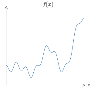
One of the most striking facts about neural networks is that they can compute any function at all. That is, suppose someone hands you some complicated, wiggly function, \(f(x)\):
.png?revision=1)
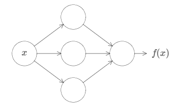
No matter what the function, there is guaranteed to be a neural network so that for every possible input, \(x\), the value \(f(x)\) (or some close approximation) is output from the network, e.g.:
.png?revision=1)
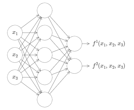
This result holds even if the function has many inputs, \(f=f(x_1,…,x_m)\), and many outputs. For instance, here's a network computing a function with \(m=3\) inputs and \(n=2\) outputs:
.png?revision=1)
This result tells us that neural networks have a kind of universality. No matter what function we want to compute, we know that there is a neural network which can do the job.
What's more, this universality theorem holds even if we restrict our networks to have just a single layer intermediate between the input and the output neurons - a so-called single hidden layer. So even very simple network architectures can be extremely powerful.
The universality theorem is well known by people who use neural networks. But why it's true is not so widely understood. Most of the explanations available are quite technical. For instance, one of the original papers proving the result*
*Approximation by superpositions of a sigmoidal function, by George Cybenko (1989). The result was very much in the air at the time, and several groups proved closely related results. Cybenko's paper contains a useful discussion of much of that work. Another important early paper is Multilayer feedforward networks are universal approximators, by Kurt Hornik, Maxwell Stinchcombe, and Halbert White (1989). This paper uses the Stone-Weierstrass theorem to arrive at similar results. did so using the Hahn-Banach theorem, the Riesz Representation theorem, and some Fourier analysis. If you're a mathematician the argument is not difficult to follow, but it's not so easy for most people. That's a pity, since the underlying reasons for universality are simple and beautiful.
In this chapter I give a simple and mostly visual explanation of the universality theorem. We'll go step by step through the underlying ideas. You'll understand why it's true that neural networks can compute any function. You'll understand some of the limitations of the result. And you'll understand how the result relates to deep neural networks.
To follow the material in the chapter, you do not need to have read earlier chapters in this book. Instead, the chapter is structured to be enjoyable as a self-contained essay. Provided you have just a little basic familiarity with neural networks, you should be able to follow the explanation. I will, however, provide occasional links to earlier material, to help fill in any gaps in your knowledge.
Universality theorems are a commonplace in computer science, so much so that we sometimes forget how astonishing they are. But it's worth reminding ourselves: the ability to compute an arbitrary function is truly remarkable. Almost any process you can imagine can be thought of as function computation. Consider the problem of naming a piece of music based on a short sample of the piece. That can be thought of as computing a function. Or consider the problem of translating a Chinese text into English. Again, that can be thought of as computing a function*
*Actually, computing one of many functions, since there are often many acceptable translations of a given piece of text.
Or consider the problem of taking an mp4 movie file and generating a description of the plot of the movie, and a discussion of the quality of the acting. Again, that can be thought of as a kind of function computation*
*Ditto the remark about translation and there being many possible functions.
Universality means that, in principle, neural networks can do all these things and many more.
Of course, just because we know a neural network exists that can (say) translate Chinese text into English, that doesn't mean we have good techniques for constructing or even recognizing such a network. This limitation applies also to traditional universality theorems for models such as Boolean circuits. But, as we've seen earlier in the book, neural networks have powerful algorithms for learning functions. That combination of learning algorithms + universality is an attractive mix. Up to now, the book has focused on the learning algorithms. In this chapter, we focus on universality, and what it means.
Two caveats
Before explaining why the universality theorem is true, I want to mention two caveats to the informal statement "a neural network can compute any function".
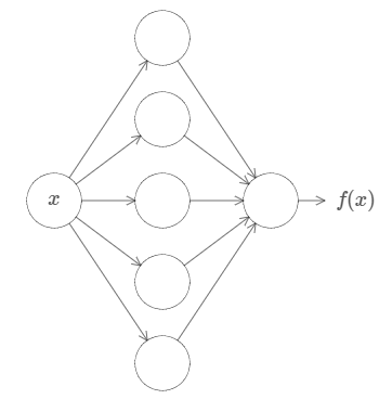
First, this doesn't mean that a network can be used to exactly compute any function. Rather, we can get an approximation that is as good as we want. By increasing the number of hidden neurons we can improve the approximation. For instance, earlier I illustrated a network computing some function \(f(x)\) using three hidden neurons. For most functions only a low-quality approximation will be possible using three hidden neurons. By increasing the number of hidden neurons (say, to five) we can typically get a better approximation:
.png?revision=1)
And we can do still better by further increasing the number of hidden neurons.
To make this statement more precise, suppose we're given a function \(f(x)\) which we'd like to compute to within some desired accuracy \(ϵ>0\). The guarantee is that by using enough hidden neurons we can always find a neural network whose output \(g(x)\) satisfies \(|g(x)−f(x)|<ϵ\), for all inputs \(x\). In other words, the approximation will be good to within the desired accuracy for every possible input.
The second caveat is that the class of functions which can be approximated in the way described are the continuous functions. If a function is discontinuous, i.e., makes sudden, sharp jumps, then it won't in general be possible to approximate using a neural net. This is not surprising, since our neural networks compute continuous functions of their input. However, even if the function we'd really like to compute is discontinuous, it's often the case that a continuous approximation is good enough. If that's so, then we can use a neural network. In practice, this is not usually an important limitation.
Summing up, a more precise statement of the universality theorem is that neural networks with a single hidden layer can be used to approximate any continuous function to any desired precision. In this chapter we'll actually prove a slightly weaker version of this result, using two hidden layers instead of one. In the problems I'll briefly outline how the explanation can, with a few tweaks, be adapted to give a proof which uses only a single hidden layer.


