5.2: Wolfram’s experiment

Last updated
Save as PDF

Page ID: 46609

\( \newcommand{\vecs}[1]{\overset { \scriptstyle \rightharpoonup} {\mathbf{#1}} } \) \( \newcommand{\vecd}[1]{\overset{-\!-\!\rightharpoonup}{\vphantom{a}\smash {#1}}} \)\(\newcommand{\id}{\mathrm{id}}\) \( \newcommand{\Span}{\mathrm{span}}\) \( \newcommand{\kernel}{\mathrm{null}\,}\) \( \newcommand{\range}{\mathrm{range}\,}\) \( \newcommand{\RealPart}{\mathrm{Re}}\) \( \newcommand{\ImaginaryPart}{\mathrm{Im}}\) \( \newcommand{\Argument}{\mathrm{Arg}}\) \( \newcommand{\norm}[1]{\| #1 \|}\) \( \newcommand{\inner}[2]{\langle #1, #2 \rangle}\) \( \newcommand{\Span}{\mathrm{span}}\) \(\newcommand{\id}{\mathrm{id}}\) \( \newcommand{\Span}{\mathrm{span}}\) \( \newcommand{\kernel}{\mathrm{null}\,}\) \( \newcommand{\range}{\mathrm{range}\,}\) \( \newcommand{\RealPart}{\mathrm{Re}}\) \( \newcommand{\ImaginaryPart}{\mathrm{Im}}\) \( \newcommand{\Argument}{\mathrm{Arg}}\) \( \newcommand{\norm}[1]{\| #1 \|}\) \( \newcommand{\inner}[2]{\langle #1, #2 \rangle}\) \( \newcommand{\Span}{\mathrm{span}}\)\(\newcommand{\AA}{\unicode[.8,0]{x212B}}\)

In the early 1980s Stephen Wolfram published a series of papers presenting a systematic study of 1-D CAs. He identified four categories of behavior, each more interesting than the last. You can read one of these papers, “Statistical mechanics of cellular automata," at http://thinkcomplex.com/ca.

In Wolfram’s experiments, the cells are arranged in a lattice (which you might remember from Section 3.2) where each cell is connected to two neighbors. The lattice can be finite, infinite, or arranged in a ring.

The rules that determine how the system evolves in time are based on the notion of a “neighborhood”, which is the set of cells that determines the next state of a given cell. Wolfram’s experiments use a 3-cell neighborhood: the cell itself and its two neighbors.

In these experiments, the cells have two states, denoted 0 and 1 or “off" and “on". A rule can be summarized by a table that maps from the state of the neighborhood (a tuple of three states) to the next state of the center cell. The following table shows an example:

prev	111	110	101	100	011	010	001	000
next	0	0	1	1	0	0	1	0

The first row shows the eight states a neighborhood can be in. The second row shows the state of the center cell during the next time step. As a concise encoding of this table, Wolfram suggested reading the bottom row as a binary number; because 00110010 in binary is 50 in decimal, Wolfram calls this CA “Rule 50”.

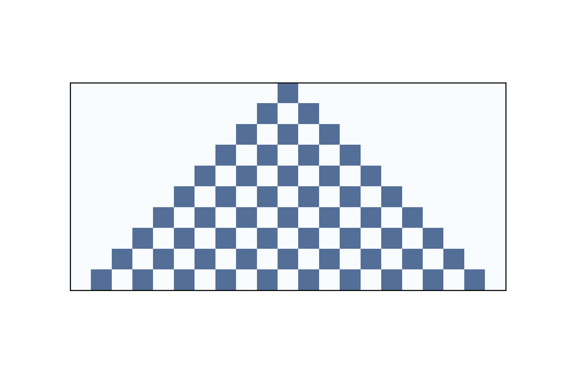
Figure \(\PageIndex{1}\): Rule 50 after 10 time steps.

Figure \(\PageIndex{1}\) shows the effect of Rule 50 over 10 time steps. The first row shows the state of the system during the first time step; it starts with one cell “on” and the rest “off”. The second row shows the state of the system during the next time step, and so on.

The triangular shape in the figure is typical of these CAs; is it a consequence of the shape of the neighborhood. In one time step, each cell influences the state of one neighbor in either direction. During the next time step, that influence can propagate one more cell in each direction. So each cell in the past has a “triangle of influence” that includes all of the cells that can be affected by it.