
7.2: Reaction-diffusion
- Page ID
- 46631

Now let’s add a second chemical. I’ll define a new object, ReactionDiffusion, that contains two arrays, one for each chemical:
class ReactionDiffusion(Cell2D):

    def __init__(self, n, m, params, noise=0.1):
        self.params = params
        self.array = np.ones((n, m), dtype=float)
        self.array2 = noise * np.random.random((n, m))
        add_island(self.array2)
n and m are the number of rows and columns in the array. params is a tuple of parameters, which I explain below.
array represents the concentration of the first chemical, A; the NumPy function ones initializes it to 1 everywhere. The data type float indicates that the elements of A are floating-point values.
array2 represents the concentration of B, which is initialized with random values between 0 and noise, which is 0.1 by default. Then add_island adds an island of higher concentration in the middle:
def add_island(a, height=0.1):
    n, m = a.shape
    radius = min(n, m) // 20
    i = n//2
    j = m//2
    a[i-radius:i+radius, j-radius:j+radius] += height
The radius of the island is one twentieth of n or m, whichever is smaller. The height of the island is height, with the default value 0.1.
Here is the step function that updates the arrays:
def step(self):
    A = self.array
    B = self.array2
    ra, rb, f, k = self.params

    cA = correlate2d(A, self.kernel, **self.options)
    cB = correlate2d(B, self.kernel, **self.options)

    reaction = A * B**2
    self.array += ra * cA - reaction + f * (1-A)
    self.array2 += rb * cB + reaction - (f+k) * B
The parameters are
ra:- The diffusion rate of
A(analogous torin the previous section). rb:- The diffusion rate of
B. In most versions of this model,rbis about half ofra. f:- The “feed” rate, which controls how quickly
Ais added to the system. k:- The “kill” rate, which controls how quickly
Bis removed from the system.
Now let’s look more closely at the update statements:
reaction = A * B**2
self.array += ra * cA - reaction + f * (1-A)
self.array2 += rb * cB + reaction - (f+k) * B
The arrays cA and cB are the result of applying a diffusion kernel to A and B. Multiplying by ra and rb yields the rate of diffusion into or out of each cell.
The term A * B**2 represents the rate that A and B react with each other. Assuming that the reaction consumes A and produces B, we subtract this term in the first equation and add it in the second.
The term f * (1-A) determines the rate that A is added to the system. Where A is near 0, the maximum feed rate is f. Where A approaches 1, the feed rate drops off to zero.
Finally, the term (f+k) * B determines the rate that B is removed from the system. As B approaches 0, this rate goes to zero.
As long as the rate parameters are not too high, the values of A and B usually stay between 0 and 1.
f=0.035 and k=0.057 after 1000, 2000, and 4000 steps.With different parameters, this model can produce patterns similar to the stripes and spots on a variety of animals. In some cases, the similarity is striking, especially when the feed and kill parameters vary in space.
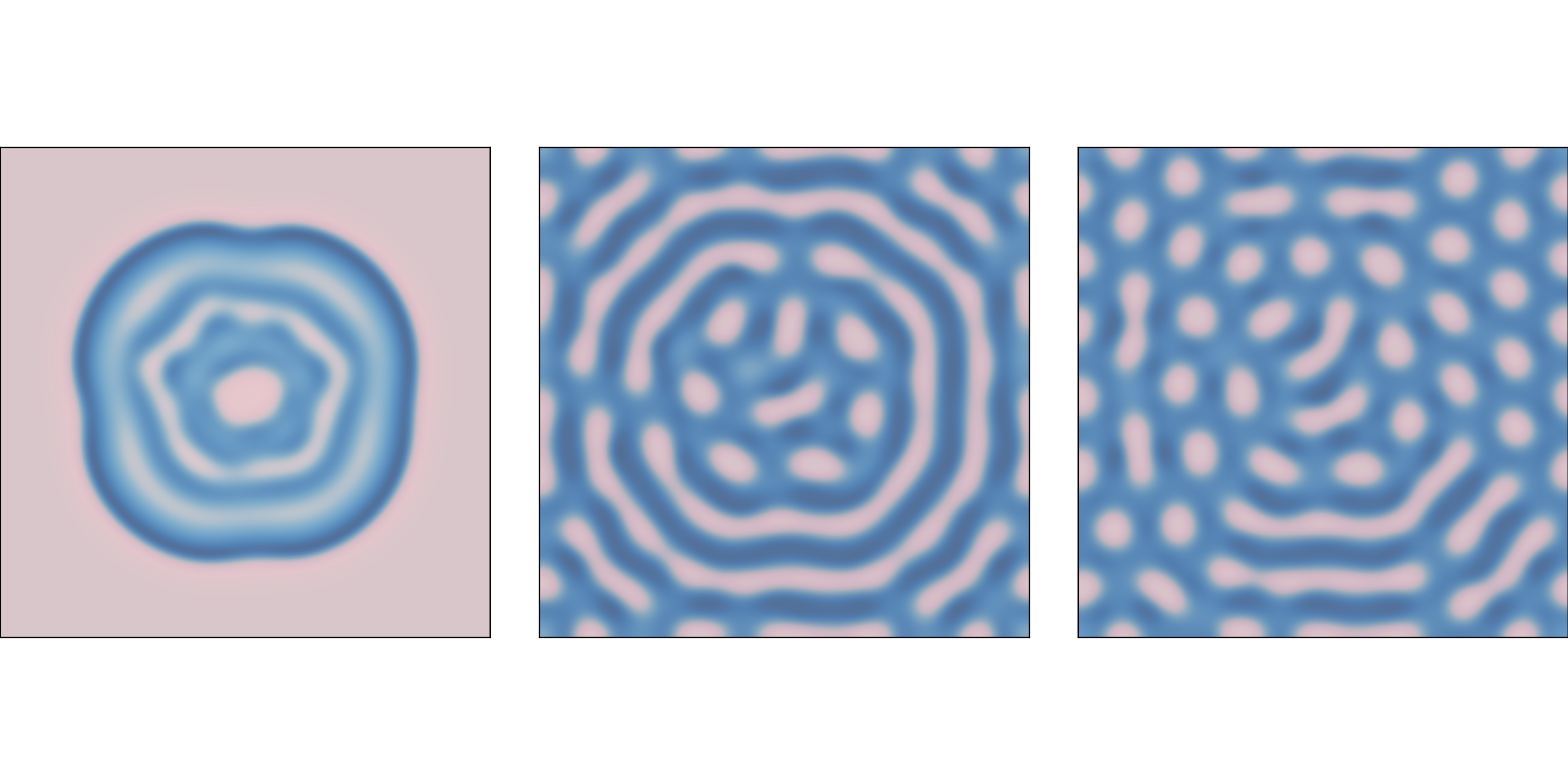
For all simulations in this section, ra=0.5 and rb=0.25.
Figure \(\PageIndex{1}\) shows results with f=0.035 and k=0.057, with the concentration of B shown in darker colors. With these parameters, the system evolves toward a stable configuration with light spots of A on a dark background of B.
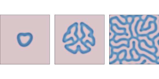
f=0.055 and k=0.062 after 1000, 2000, and 4000 steps.Figure \(\PageIndex{2}\) shows results with f=0.055 and k=0.062, which yields a coral-like pattern of B on a background of A.
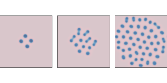
f=0.039 and k=0.065 after 1000, 2000, and 4000 steps.Figure \(\PageIndex{3}\) shows results with f=0.039 and k=0.065. These parameters produce spots of B that grow and divide in a process that resembles mitosis, ending with a stable pattern of equally-spaced spots.
Since 1952, observations and experiments have provided some support for Turing’s conjecture. At this point it seems likely, but not yet proven, that many animal patterns are actually formed by reaction-diffusion processes of some kind.