2.6: Generating ER graphs

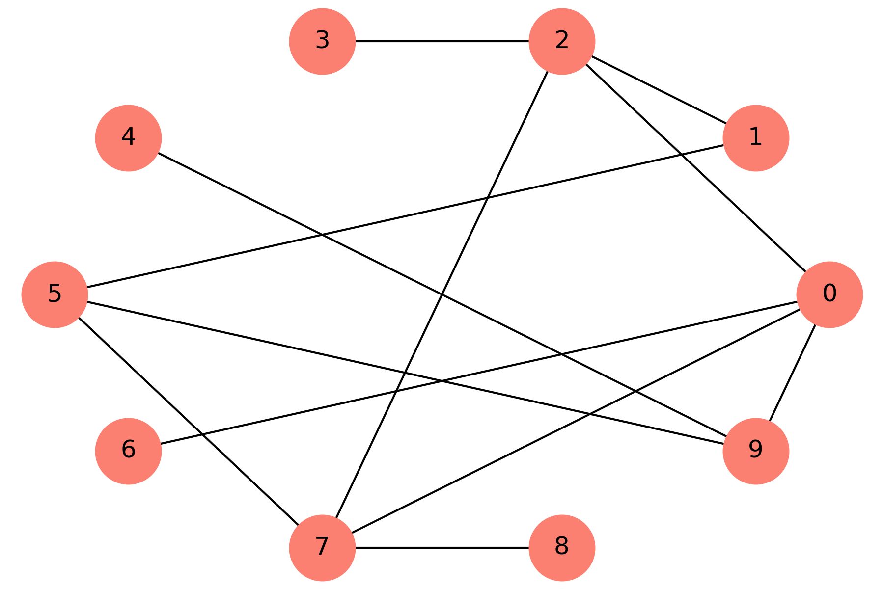
Figure \(\PageIndex{1}\): An ER graph with n=10 and p=0.3.

The ER graph G(n, p) contains n nodes, and each pair of nodes is connected by an edge with probability p. Generating an ER graph is similar to generating a complete graph.

The following generator function enumerates all possible edges and chooses which ones should be added to the graph:

def random_pairs(nodes, p): 
    for edge in all_pairs(nodes): 
        if flip(p): 
            yield edge

random_pairs uses flip:

def flip(p): 
    return np.random.random() < p

This is the first example we’re seen that uses NumPy. Following convention, I import numpy as np. NumPy provides a module named random, which provides a method named random, which returns a number between 0 and 1, uniformly distributed.

So flip returns True with the given probability, p, and False with the complementary probability, 1-p.

Finally, make_random_graph generates and returns the ER graph G(n, p):

def make_random_graph(n, p): 
    G = nx.Graph() 
    nodes = range(n) 
    G.add_nodes_from(nodes) 
    G.add_edges_from(random_pairs(nodes, p)) 
    return G

make_random_graph is almost identical to make_complete_graph; the only difference is that it uses random_pairs instead of all_pairs.

Here’s an example with p=0.3:

random_graph = make_random_graph(10, 0.3)

Figure \(\PageIndex{1}\) shows the result. This graph turns out to be connected; in fact, most ER graphs with n=10 and p=0.3 are connected. In the next section, we’ll see how many.