2.2: Warm up- a fast matrix-based approach to computing the output from a neural network

Before discussing backpropagation, let's warm up with a fast matrix-based algorithm to compute the output from a neural network. We actually already briefly saw this algorithm near the end of the last chapter, but I described it quickly, so it's worth revisiting in detail. In particular, this is a good way of getting comfortable with the notation used in backpropagation, in a familiar context.

Let's begin with a notation which lets us refer to weights in the network in an unambiguous way. We'll use \(w_{jk}^l\) to denote the weight for the connection from the \(k^{th}\) neuron in the \((l−1)^{th}\) layer to the \(j^{th}\) neuron in the \(l^{th}\) layer. So, for example, the diagram below shows the weight on a connection from the fourth neuron in the second layer to the second neuron in the third layer of a network:

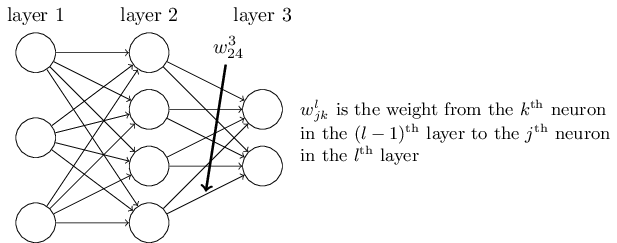
This notation is cumbersome at first, and it does take some work to master. But with a little effort you'll find the notation becomes easy and natural. One quirk of the notation is the ordering of the \(j\) and \(k\) indices. You might think that it makes more sense to use \(j\) to refer to the input neuron, and \(k\) to the output neuron, not vice versa, as is actually done. I'll explain the reason for this quirk below.

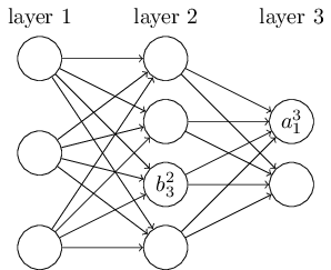
We use a similar notation for the network's biases and activations. Explicitly, we use \(b_{j}^l\) for the bias of the \(j^{th}\) neuron in the \(l^{th}\) layer. And we use \(a_{j}^l\) for the activation of the \(j^{th}\) neuron in the \(l^{th}\) layer. The following diagram shows examples of these notations in use:

With these notations, the activation \(a_{j}^l\) of the \(j^{th}\) neuron in the \(l^{th}\) layer is related to the activations in the \((l−1)^{th}\) layer by the equation (compare Equation (1.3.2) and surrounding discussion in the last chapter)

\[ a_{j}^l = σ \Big(\sum_k w_{jk}^l a_{k}^{l-1} + b_{j}^l\Big), \]

where the sum is over all neurons \(k\) in the \((l−1)^{th}\) layer. To rewrite this expression in a matrix form we define a weight matrix \(w^l\) for each layer, \(l\). The entries of the weight matrix \(w^l\) are just the weights connecting to the \(l^th\) layer of neurons, that is, the entry in the \(j^{th}\) and \(k^{th}\) column is \(w_{jk}^l\). Similarly, for each layer \(l\) we define a bias vector, \(b^l\). You can probably guess how this works - the components of the bias vector are just the values \(b_{j}^l\), one component for each neuron in the \(l^{th}\) layer. And finally, we define an activation vector \(a^l\) whose components are the activations \(a_{j}^l\).

The last ingredient we need to rewrite (2.2.1) in a matrix form is the idea of vectorizing a function such as σσ. We met vectorization briefly in the last chapter, but to recap, the idea is that we want to apply a function such as \(σ\) to every element in a vector \(v\). We use the obvious notation \(σ(v)\) to denote this kind of elementwise application of a function. That is, the components of \(σ(v)\) are just \(σ(v)_j = σ(v_j)\). As an example, if we have the function \(f(x) = x^2\) then the vectorized form of ff has the effect

\[ f\bigg(\begin{bmatrix} 2 \\ 3 \end{bmatrix}\bigg) = \begin{bmatrix} f(2) \\ f(3) \end{bmatrix} = \begin{bmatrix} 4 \\ 9 \end{bmatrix}, \]

that is, the vectorized ff just squares every element of the vector.

With these notations in mind, Equation (2.2.1) can be rewritten in the beautiful and compact vectorized form

\[ a^l = σ(w^l a^{l-1} + b^l). \]

This expression gives us a much more global way of thinking about how the activations in one layer relate to activations in the previous layer: we just apply the weight matrix to the activations, then add the bias vector, and finally apply the \(σ\) function*

*By the way, it's this expression that motivates the quirk in the \(w^l_{jk}\) notation mentioned earlier. If we used \(j\) to index the input neuron, and \(k\) to index the output neuron, then we'd need to replace the weight matrix in Equation (2.2.2) by the transpose of the weight matrix. That's a small change, but annoying, and we'd lose the easy simplicity of saying (and thinking) "apply the weight matrix to the activations".

That global view is often easier and more succinct (and involves fewer indices!) than the neuron-by-neuron view we've taken to now. Think of it as a way of escaping index hell, while remaining precise about what's going on. The expression is also useful in practice, because most matrix libraries provide fast ways of implementing matrix multiplication, vector addition, and vectorization. Indeed, the code in the last chapter made implicit use of this expression to compute the behaviour of the network.

When using Equation (2.2.3) to compute \(a^l\), we compute the intermediate quantity \(z^l ≡ w^l a^{l−1} + b^l\) along the way. This quantity turns out to be useful enough to be worth naming: we call \(z^l\) the weighted input to the neurons in layer \(l\). We'll make considerable use of the weighted input \(z^l\) later in the chapter. Equation (2.2.3) is sometimes written in terms of the weighted input, as \(a^l=σ(z^l)\). It's also worth noting that \(z^l\) has components \(z^l_j =\sum_k w^l_{jk} a^{l−1}_k + b^l_j\), that is, \(z^l_j\) is just the weighted input to the activation function for neuron \(j\) in layer \(l\).

The two assumptions we need about the cost function

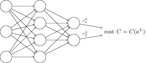
The goal of backpropagation is to compute the partial derivatives \(∂C/∂w\) and \(∂C/∂b\) of the cost function \(C\) with respect to any weight \(w\) or bias \(b\) in the network. For backpropagation to work we need to make two main assumptions about the form of the cost function. Before stating those assumptions, though, it's useful to have an example cost function in mind. We'll use the quadratic cost function from last chapter (c.f. Equation (1.6.1)). In the notation of the last section, the quadratic cost has the form

\[ C =\frac{1}{2n} \sum_x {∥y(x)−a^L (x)∥}^2 \]

where: \(n\) is the total number of training examples; the sum is over individual training examples, \(x\); \(y = y(x)\) is the corresponding desired output; \(L\) denotes the number of layers in the network; and \(a^L =a^L (x)\) is the vector of activations output from the network when \(x\) is input.

Okay, so what assumptions do we need to make about our cost function, \(C\), in order that backpropagation can be applied? The first assumption we need is that the cost function can be written as an average \(C = \frac{1}{n}\sum_x C_x\) over cost functions \(Cx\) for individual training examples, \(x\). This is the case for the quadratic cost function, where the cost for a single training example is \(C_x = \frac{1}{2} {∥y−a^L∥}^2\). This assumption will also hold true for all the other cost functions we'll meet in this book.

The reason we need this assumption is because what backpropagation actually lets us do is compute the partial derivatives \(∂Cx/∂w\) and \(∂Cx/∂b\) for a single training example. We then recover \(∂C/∂w\) and \(∂C/∂b\) by averaging over training examples. In fact, with this assumption in mind, we'll suppose the training example \(x\) has been fixed, and drop the x subscript, writing the cost \(C_x\) as \(C\). We'll eventually put the \(x\) back in, but for now it's a notational nuisance that is better left implicit.

The second assumption we make about the cost is that it can be written as a function of the outputs from the neural network:

For example, the quadratic cost function satisfies this requirement, since the quadratic cost for a single training example \(x\) may be written as

\[ C = \frac{1}{2} {∥y−a^L∥}^2 = \frac{1}{2} \sum_j {(y_j−a^L_j)}^2, \]

and thus is a function of the output activations. Of course, this cost function also depends on the desired output \(y\), and you may wonder why we're not regarding the cost also as a function of \(y\). Remember, though, that the input training example \(x\) is fixed, and so the output \(y\) is also a fixed parameter. In particular, it's not something we can modify by changing the weights and biases in any way, i.e., it's not something which the neural network learns. And so it makes sense to regard \(C\) as a function of the output activations \(a^L\) alone, with \(y\) merely a parameter that helps define that function.

The Hadamard product, \(s⊙t\)

The backpropagation algorithm is based on common linear algebraic operations - things like vector addition, multiplying a vector by a matrix, and so on. But one of the operations is a little less commonly used. In particular, suppose ss and tt are two vectors of the same dimension. Then we use \(s⊙t\) to denote the elementwise product of the two vectors. Thus the components of \(s⊙t\) are just \((s⊙t)_j = s_jt_j\). As an example,

\[ \begin{bmatrix} 1 \\ 2 \end{bmatrix} ⊙ \begin{bmatrix} 3 \\ 4 \end{bmatrix} = \begin{bmatrix} 1*3 \\ 2*4 \end{bmatrix} = \begin{bmatrix} 3 \\ 8 \end{bmatrix} \]

This kind of elementwise multiplication is sometimes called the Hadamard product or Schur product. We'll refer to it as the Hadamard product. Good matrix libraries usually provide fast implementations of the Hadamard product, and that comes in handy when implementing backpropagation.

The four fundamental equations behind backpropagation

Backpropagation is about understanding how changing the weights and biases in a network changes the cost function. Ultimately, this means computing the partial derivatives \(∂C/∂w^l_{jk}\) and \(∂C/∂b^l_j\). But to compute those, we first introduce an intermediate quantity, \(δ^l_j\), which we call the error in the \(j^th\) neuron in the \(l^th\) layer. Backpropagation will give us a procedure to compute the error \(δ^l_j\), and then will relate \(δ^l_j\) to \(∂C/∂w^l_{jk}\) and \(∂C/∂b^l_j\).

To understand how the error is defined, imagine there is a demon in our neural network:

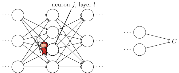
The demon sits at the \(j^th\) neuron in layer \(l\). As the input to the neuron comes in, the demon messes with the neuron's operation. It adds a little change \(Δz^l_j\) to the neuron's weighted input, so that instead of outputting \(σ(z^l_j)\), the neuron instead outputs \(σ(z^l_j + Δz^l_j)\). This change propagates through later layers in the network, finally causing the overall cost to change by an amount \(\frac{∂C}{∂z^l_j} Δz^l_j\).

Now, this demon is a good demon, and is trying to help you improve the cost, i.e., they're trying to find a \(Δz^l_j\) which makes the cost smaller. Suppose \(\frac{∂C}{∂z^l_j}\) has a large value (either positive or negative). Then the demon can lower the cost quite a bit by choosing \(Δz^l_j\) to have the opposite sign to \(\frac{∂C}{∂z^l_j}\). By contrast, if \(\frac{∂C}{∂z^l_j}\) is close to zero, then the demon can't improve the cost much at all by perturbing the weighted input \(z^l_j\). So far as the demon can tell, the neuron is already pretty near optimal*

*This is only the case for small changes \(Δz^l_j\), of course. We'll assume that the demon is constrained to make such small changes.

And so there's a heuristic sense in which \(\frac{∂C}{∂z^l_j}\) is a measure of the error in the neuron.

Motivated by this story, we define the error \(δ^l_j\) of neuron \(j\) in layer \(l\) by

\[ δ^l_j ≡ \frac{∂C}{∂z^l_j} \]

As per our usual conventions, we use \(δ^l\) to denote the vector of errors associated with layer \(l\). Backpropagation will give us a way of computing \(δ^l\) for every layer, and then relating those errors to the quantities of real interest, \(\frac{∂C}{∂w^l_{jk}}\) and \(\frac{∂C}{∂b^l_j}\).

You might wonder why the demon is changing the weighted input \(z^l_j\). Surely it'd be more natural to imagine the demon changing the output activation \(a^l_j\), with the result that we'd be using \(\frac{∂C}{∂a^l_j}\) as our measure of error. In fact, if you do this things work out quite similarly to the discussion below. But it turns out to make the presentation of backpropagation a little more algebraically complicated. So we'll stick with \(δ^l_j = \frac{∂C}{∂z^l_j}\) as our measure of error*

*In classification problems like MNIST the term "error" is sometimes used to mean the classification failure rate. E.g., if the neural net correctly classifies 96.0 percent of the digits, then the error is 4.0 percent. Obviously, this has quite a different meaning from our \(δ\) vectors. In practice, you shouldn't have trouble telling which meaning is intended in any given usage.

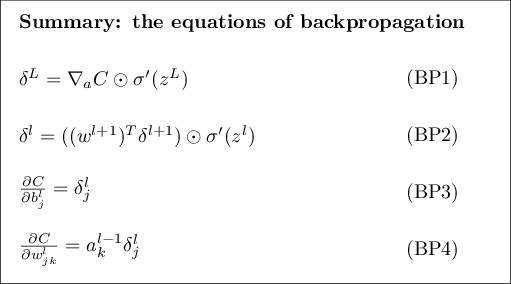
Plan of attack: Backpropagation is based around four fundamental equations. Together, those equations give us a way of computing both the error \(δ^l\) and the gradient of the cost function. I state the four equations below. Be warned, though: you shouldn't expect to instantaneously assimilate the equations. Such an expectation will lead to disappointment. In fact, the backpropagation equations are so rich that understanding them well requires considerable time and patience as you gradually delve deeper into the equations. The good news is that such patience is repaid many times over. And so the discussion in this section is merely a beginning, helping you on the way to a thorough understanding of the equations.

Here's a preview of the ways we'll delve more deeply into the equations later in the chapter: I'll give a short proof of the equations, which helps explain why they are true; we'll restate the equations in algorithmic form as pseudocode, and see how the pseudocode can be implemented as real, running Python code; and, in the final section of the chapter, we'll develop an intuitive picture of what the backpropagation equations mean, and how someone might discover them from scratch. Along the way we'll return repeatedly to the four fundamental equations, and as you deepen your understanding those equations will come to seem comfortable and, perhaps, even beautiful and natural.

An equation for the error in the output layer, \(δ^L\) The components of \(δ^L\) are given by

\[ δ^L_j = \frac{∂C}{∂a^L_j} σ′(z^L_j) \]

This is a very natural expression. The first term on the right, \(\frac{∂C}{∂a^L_j}\), just measures how fast the cost is changing as a function of the \(j^th\) output activation. If, for example, \(C\) doesn't depend much on a particular output neuron, \(j\), then \(δ^L_j\) will be small, which is what we'd expect. The second term on the right, \(σ′(z^L_j)\), measures how fast the activation function \(σ\) is changing at \(z^L_j\).

Notice that everything in (BP1) is easily computed. In particular, we compute \(z^L_j\) while computing the behaviour of the network, and it's only a small additional overhead to compute \(σ′(z^L_j)\). The exact form of \(\frac{∂C}{∂a^L_j}\) will, of course, depend on the form of the cost function. However, provided the cost function is known there should be little trouble computing \(\frac{∂C}{∂a^L_j}\). For example, if we're using the quadratic cost function then \(C =\frac{1}{2}\sum_j{(y_j−a^L_j)}^2\), and so \(\frac{∂C}{∂a^L_j} = (a^L_j − y_j)\), which obviously is easily computable.

Equation (BP1) is a componentwise expression for \(δ^L\). It's a perfectly good expression, but not the matrix-based form we want for backpropagation. However, it's easy to rewrite the equation in a matrix-based form, as

\[ δ^L = ∇_a C⊙σ′(z^L). \]

Here, \(∇_aC\) is defined to be a vector whose components are the partial derivatives \(\frac{∂C}{∂a^L_j}\). You can think of \(∇_aC\) as expressing the rate of change of \(C\) with respect to the output activations. It's easy to see that Equations (BP1a) and (BP1) are equivalent, and for that reason from now on we'll use (BP1) interchangeably to refer to both equations. As an example, in the case of the quadratic cost we have \(∇_aC = (a^L−y)\), and so the fully matrix-based form of (BP1)becomes

\[ δ^L = (a^L−y)⊙σ′(z^L) \]

As you can see, everything in this expression has a nice vector form, and is easily computed using a library such as Numpy.

An equation for the error \(δ^l\) in terms of the error in the next layer, \(δ^{l+1}\): In particular

\[ δ^l = ((w^{l+1})^T δ^{l+1})⊙σ′(z^l) \]

where \((w^{l+1})^T\) is the transpose of the weight matrix \(w^{l+1}\) for the \((l+1)^{th}\) layer. This equation appears complicated, but each element has a nice interpretation. Suppose we know the error \(δ^{l+1}\) at the \(l+1^{th}\) layer. When we apply the transpose weight matrix, \((w^{l+1})^T\), we can think intuitively of this as moving the error backward through the network, giving us some sort of measure of the error at the output of the \(l^{th}\) layer. We then take the Hadamard product \(⊙σ′(z^l)\). This moves the error backward through the activation function in layer ll, giving us the error \(δ^l\) in the weighted input to layer \(l\).

By combining (BP2) with (BP1) we can compute the error \(δ^l\) for any layer in the network. We start by using (BP1) to compute \(δ^L\), then apply Equation (BP2) to compute \(δ^{L−1}\), then Equation (BP2) again to compute \(δ^{L−2}\), and so on, all the way back through the network.

An equation for the rate of change of the cost with respect to any bias in the network: In particular:

\[ \frac{∂C}{∂b^L_j} = δ^l_j \]

That is, the error \(δ^l_j\) is exactly equal to the rate of change \(\frac{∂C}{∂b^L_j}\) . This is great news, since (BP1) and (BP2) have already told us how to compute \(δ^l_j\). We can rewrite (BP3) in shorthand as

\[ \frac{∂C}{∂b} = δ \]

where it is understood that \(δ\) is being evaluated at the same neuron as the bias \(b\).

An equation for the rate of change of the cost with respect to any weight in the network: In particular:

\[ \frac{∂C}{∂w^L_{jk}} = a^{l−1}_k δ^l_j \]

This tells us how to compute the partial derivatives \(\frac{∂C}{∂w^L_{jk}}\) in terms of the quantities \(δ^l\) and \(a^{l−1}\), which we already know how to compute. The equation can be rewritten in a less index-heavy notation as

\[ \frac{∂C}{∂w} = a_{in}δ_{out} \]

where it's understood that \(a_{in}\) is the activation of the neuron input to the weight \(w\), and \(δ_{out}\) is the error of the neuron output from the weight \(w\). Zooming in to look at just the weight \(w\), and the two neurons connected by that weight, we can depict this as:

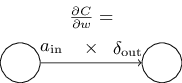
A nice consequence of Equation (2.2.15) is that when the activation \(a_{in}\) is small, \(a_{in} ≈ 0\) , the gradient term \(\frac{∂C}{∂w}\) will also tend to be small. In this case, we'll say the weight learns slowly, meaning that it's not changing much during gradient descent. In other words, one consequence of (BP4) is that weights output from low-activation neurons learn slowly.

There are other insights along these lines which can be obtained from (BP1)-(BP4). Let's start by looking at the output layer. Consider the term \(σ′(z^L_j)\) in (BP1). Recall from the graph of the sigmoid function in the last chapter that the \(σ\) function becomes very flat when \(σ(z^L_j)\) is approximately \(0\) or \(1\). When this occurs we will have \(σ′(z^L_j) ≈ 0\). And so the lesson is that a weight in the final layer will learn slowly if the output neuron is either low activation \((≈0)\) or high activation \((≈1)\). In this case it's common to say the output neuron has saturated and, as a result, the weight has stopped learning (or is learning slowly). Similar remarks hold also for the biases of output neuron.

We can obtain similar insights for earlier layers. In particular, note the \(σ′(z^l)\) term in (BP2). This means that \(δ^l_j\) is likely to get small if the neuron is near saturation. And this, in turn, means that any weights input to a saturated neuron will learn slowly*

*This reasoning won't hold if \(w^{l+1^T} δ^{l+1}\) has large enough entries to compensate for the smallness of \(σ′(z^l_j)σ′(zjl)\). But I'm speaking of the general tendency.

Summing up, we've learnt that a weight will learn slowly if either the input neuron is low-activation, or if the output neuron has saturated, i.e., is either high- or low-activation.

None of these observations is too greatly surprising. Still, they help improve our mental model of what's going on as a neural network learns. Furthermore, we can turn this type of reasoning around. The four fundamental equations turn out to hold for any activation function, not just the standard sigmoid function (that's because, as we'll see in a moment, the proofs don't use any special properties of \(σ\)). And so we can use these equations to design activation functions which have particular desired learning properties. As an example to give you the idea, suppose we were to choose a (non-sigmoid) activation function \(σ\) so that \(σ′\) is always positive, and never gets close to zero. That would prevent the slow-down of learning that occurs when ordinary sigmoid neurons saturate. Later in the book we'll see examples where this kind of modification is made to the activation function. Keeping the four equations (BP1)-(BP4) in mind can help explain why such modifications are tried, and what impact they can have.

Problem

• Alternate presentation of the equations of backpropagation: I've stated the equations of backpropagation (notably (BP1) and (BP2)) using the Hadamard product. This presentation may be disconcerting if you're unused to the Hadamard product. There's an alternative approach, based on conventional matrix multiplication, which some readers may find enlightening. (1) Show that (BP1) may be rewritten as

  \[ δ^L = Σ′(z^L)∇_a C, \]

  where \(Σ′(z^L)\) is a square matrix whose diagonal entries are the values \(σ′(z^L_j)\), and whose off-diagonal entries are zero. Note that this matrix acts on \(∇_a C\) by conventional matrix multiplication. (2) Show that (BP2) may be rewritten as

  \[ δ^l = Σ′(z^l)(w^{l+1})^T δ{l+1}. \]

  (3) By combining observations (1) and (2) show that

  \[ δ^l = Σ′(z^l)(w^{l+1})^T…Σ′(z^{L−1}) (w^L)^T Σ′(z^L) ∇_a C \]

• For readers comfortable with matrix multiplication this equation may be easier to understand than (BP1) and (BP2). The reason I've focused on (BP1) and (BP2) is because that approach turns out to be faster to implement numerically.

Proof of the four fundamental equations (optional)

We'll now prove the four fundamental equations (BP1)-(BP4). All four are consequences of the chain rule from multivariable calculus. If you're comfortable with the chain rule, then I strongly encourage you to attempt the derivation yourself before reading on.

Let's begin with Equation (BP1), which gives an expression for the output error, \(δ^L\). To prove this equation, recall that by definition

\[ δ^L_j = \frac{∂C}{∂z^L_j}. \]

Applying the chain rule, we can re-express the partial derivative above in terms of partial derivatives with respect to the output activations,

\[ δ^L_j = \sum_k \frac{∂C}{∂a^L_k} \frac{∂a^L_k}{∂z^L_j}, \]

where the sum is over all neurons \(k\) in the output layer. Of course, the output activation \(a^L_k\) of the \(k^{th}\) neuron depends only on the weighted input \(z^L_j\) for the \(j^{th}\) neuron when \(k = j\). And so \(∂a^L_k/∂z^L_j\) vanishes when \(k≠j\). As a result we can simplify the previous equation to

\[ δ^L_j = \frac{∂C}{∂a^L_j} \frac{∂a^L_j}{∂z^L_j}. \]

Recalling that \(a^L_j = σ(z^L_j)\) the second term on the right can be written as \(σ′(z^L_j)\), and the equation becomes

\[ δ^L_j = \frac{∂C}{∂a^L_j} σ′(z^L_j), \]

which is just (BP1), in component form.

Next, we'll prove (BP2), which gives an equation for the error \(δ^l\) in terms of the error in the next layer, \(δ^{l+1}\). To do this, we want to rewrite \(δ^l_j = ∂C/∂z^l_j\) in terms of \(δ^{l+1}_k = ∂C/∂z{l+1}_k\). We can do this using the chain rule,

\[\begin{aligned} δ^l_j & = \frac{∂C}{∂z^l_j}\\ &= \sum_k \frac{∂C}{∂z^{l+1}_k} \frac{∂z^{l+1}_k}{∂z^l_j} \\ &= \sum_k \frac{∂z^{l+1}_k}{∂z^l_j} δ^{l+1}_k, \end{aligned}\]

where in the last line we have interchanged the two terms on the right-hand side, and substituted the definition of \(δ^{l+1}_k\). To evaluate the first term on the last line, note that

\[ z{l+1}_k =\sum_j w{l+1}_{kj} a^l_j + b^{l+1}_k =\sum_j w^{l+1}_{kj} σ(z^l_j) + b^{l+1}_k. \]

Differentiating, we obtain

\[ \frac{∂z^{l+1}_k}{∂z^l_j} = w^{l+1}_{kj} σ′(z^l_j). \]

Substituting back into (42) we obtain

\[ δ^l_j = \sum_k w^{l+1}_{kj} δ^{l+1}_k σ′(z^l_j). \]

This is just (BP2) written in component form.

The final two equations we want to prove are (BP3) and (BP4). These also follow from the chain rule, in a manner similar to the proofs of the two equations above. I leave them to you as an exercise.

Exercise

• Prove Equations (BP3) and (BP4).

That completes the proof of the four fundamental equations of backpropagation. The proof may seem complicated. But it's really just the outcome of carefully applying the chain rule. A little less succinctly, we can think of backpropagation as a way of computing the gradient of the cost function by systematically applying the chain rule from multi-variable calculus. That's all there really is to backpropagation - the rest is details.