
5.6: Three-Dimensional Homogeneous Coordinates
- Page ID
- 9980

We now consider the storage and manipulation of three-dimensional objects. We will continue to use homogeneous coordinates so that translation can be included in composite operators. Homogeneous coordinates in three dimensions will also allow us to do perspective projections so that we can view a three-dimensional object from any point in space.
Image Representation
The three-dimensional form of the point matrix in homogeneous coordinates is
\[\mathrm{G}=\left\{\begin{array}{lllll}
x_{1} & x_{2} & x_{3} & \ldots & x_{n} \\
y_{1} & y_{2} & y_{3} & \ldots & y_{n} \\
z_{1} & z_{2} & z_{3} & \ldots & z_{n} \\
1 & 1 & 1 & \ldots & 1
\end{array}\right\} \in \mathscr{R}^{4 \times n} \nonumber \]
The line matrix \(H\) is exactly as before, pointing to pairs of columns in \(G\) to connect with lines. Any other grouping matrices for objects, etc., are also unchanged.
Image manipulations are done by a 4×4 matrix \(A\). To ensure that the fourth coordinate remains a 1, the operator \(A\) must have the structure
\[A=\left[\begin{array}{llll}
a_{11} & a_{12} & a_{13} & a_{14} \\
a_{21} & a_{22} & a_{23} & a_{24} \\
a_{31} & a_{32} & a_{33} & a_{34} \\
0 & 0 & 0 & 1
\end{array}\right] \nonumber \]
The new image has point matrix
\[\mathrm{G}_{\text {new }}=A G \nonumber \]
If the coordinates of the \(i^{th}\) point in \(G\) are \((x_i,y_i,z_i,1)\), what are the coordinates of the \(i^{th}\) point in \(\mathrm{G}_{\text {new }}=A G\) when \(A\) is as given in Equation 2?
Write down the point matrix \(G\) for the unit cube (the cube with sides of length 1, with one corner at the origin and extending in the positive direction along each axis). Draw a sketch of the cube, numbering the vertices according to their order in your point matrix. Now write down the line matrix \(H\) to complete the representation of the cube.
Left- and Right-Handed Coordinate Systems
In this book we work exclusively with right-handed coordinate systems. However, it is worth pointing out that there are two ways to arrange the axes in three dimensions. Figure 1(a) shows the usual right-handed coordinates, and the left-handed variation is shown in Figure 1(b). All possible choices of labels \(x\), \(y\), and \(z\) for the three coordinate axes can be rotated to fit one of these two figures, but no rotation will go from one to the other.
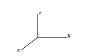 (a)
(a)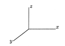 (b)
(b)Be careful to sketch a right-handed coordinate system when you are solving problems in this chapter. Some answers will not be the same for a left-handed system.
Image Transformation
Three-dimensional operations are a little more complicated than their two-dimensional counterparts. For scaling and translation we now have three independent directions, so we generalize the operators of Equation 10 from "Vector Graphics: Homogeneous Coordinates" as
\[\mathrm{S}\left(s_{x}, s_{y}, s_{z}\right)=\left\{\begin{array}{llll}
s_{x} & 0 & 0 & 0 \\
0 & s_{y} & 0 & 0 \\
0 & 0 & s_{z} & 0 \\
0 & 0 & 0 & 1
\end{array}\right\} \nonumber \]
\[\mathrm{T}\left(t_{x}, t_{y}, t_{z}\right)=\left[\begin{array}{llll}
1 & 0 & 0 & t_{x} \\
0 & 1 & 0 & t_{y} \\
0 & 0 & 1 & t_{z} \\
0 & 0 & 0 & 1
\end{array}\right] \text { . } \nonumber \]
Show that T\((−t_x,−t_y,−t_z)\) is the inverse of T\((t_x,t_y,t_z)\. T\(^{-1}\) undoes the work of \(T\).
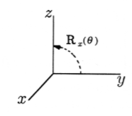
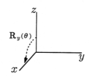
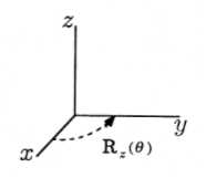
Rotation may be done about any arbitrary line in three dimensions. We will build up to the general case by first presenting the operators that rotate about the three coordinate axes. R\(_x(\theta)\) rotates by angle \(\theta\) about the x-axis, with positive \(\theta\) going from the y-axis to the z-axis, as shown in Figure 2. In a similar fashion, positive rotation about the y-axis using R\(_y(\theta)\) goes from \(z\) to \(x\), and positive rotation about the z-axis goes from \(x\) to \(y\), just as in two dimensions. We have the fundamental rotations
\[\mathrm{R}_{x}(\theta)=\left\{\begin{array}{llll}
1 & 0 & 0 & 0 \\
0 & \cos \theta & -\sin \theta & 0 \\
0 & \sin \theta & \cos \theta & 0 \\
0 & 0 & 0 & 1
\end{array}\right\} \nonumber \]
\[\mathrm{R}_{y}(\theta)=\left\{\begin{array}{llll}
\cos \theta & 0 & \sin \theta & 0 \\
0 & 1 & 0 & 0 \\
-\sin \theta & 0 & \cos \theta & 0 \\
0 & 0 & 0 & 1
\end{array}\right\} \nonumber \]
\[\mathrm{R}_{z}(\theta)=\left\{\begin{array}{llll}
\cos \theta & -\sin \theta & 0 & 0 \\
\sin \theta & \cos \theta & 0 & 0 \\
0 & 0 & 1 & 0 \\
0 & 0 & 0 & 1
\end{array}\right\} \nonumber \]
A more general rotation about any line through the origin can be constructed by composition of the three fundamental rotations. Finally, by composing translation with the fundamental rotations, we can build an operator that rotates about any arbitrary line in space.
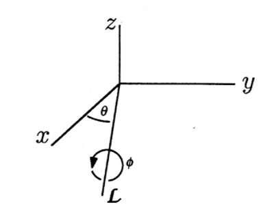
To rotate by angle \(\psi\) about the line \(\mathscr{L}\), which lies in the \(x−y\) plane in Figure 3, we would
- rotate \(\mathscr{L}\) to the x-axis with R\(_z(−\theta)\);
- rotate by \(\psi\) about the x-axis with R\(_x(\psi)\); and
- rotate back to \(\mathscr{L}\) with R\(_z(\theta)\).
The composite operation would be
\[\mathrm{A}(\theta, \varphi)=\mathrm{R}_{z}(\theta) \mathrm{R}_{x}(\varphi) \mathrm{R}_{z}(-\theta) \nonumber \]
Direction Cosines
As discussed in the chapter on Linear Algebra, a vector vv may be specified by its coordinates \((x,y,z)\) or by its length and direction. The length of \(\nu\) is ||\(\nu\)||, and the direction can be specified in terms of the three direction cosines \((\cos{\theta_x}, \cos{\theta_y}, \cos{\theta_z})\). The angle \(\theta_x\) is measured between the vector \(\nu\) and the x-axis or, equivalently, between the vector \(\nu\) and the vector \(e_x=[100]^T\). We have
\[\cos \theta_{x}=\frac{\left(\mathrm{v}, \mathrm{e}_{x}\right)}{\|\mathrm{v}\|\left\|\mathrm{e}_{x}\right\|}=\frac{x}{\|\mathrm{v}\|} \nonumber \]
Likewise, \(\theta_y\) is measured between \(\nu\) and \(e_y=[010]^T\), and \(\theta_z\) is measured between \(\nu\) and \(e_z=[001]^\). Thus
\[\cos \theta_{y}=\frac{y}{\|\mathrm{v}\|} \nonumber \]
\[\cos \theta_{z}=\frac{z}{\|v\|} \nonumber \]
The vector
\[\mathrm{u}=\left\{\begin{array}{c}
\cos \theta_{x} \\
\cos \theta_{y} \\
\cos \theta_{z}
\end{array}\right\} \nonumber \]
s a unit vector in the direction of \(\nu\), so we have
\[\mathrm{v}=\|\mathrm{v}\| \mathrm{u}=\|\mathrm{v}\|\left\{\begin{array}{l}
\cos \theta_{x} \\
\cos \theta_{y} \\
\cos \theta_{z}
\end{array}\right\} \nonumber \]
Show that \(u\) is a unit vector (i.e. 1 u||=1u||=1).
The direction cosines are useful for specifying a line in space. Instead of giving two points \(P_1\) and \(P_2\) on the line, we can give one point \(P_1\) plus the direction cosines of any vector that points along the line. One such vector is the vector from \(P_1\) to \(P_2\).
Arc tangents
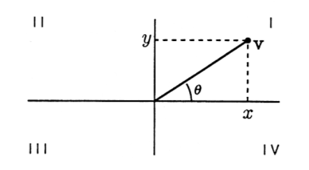
Consider a vector \(\mathrm{v}=\left\{\begin{array}{l}
x \\
y
\end{array}\right\}\) in two dimensions. We know that
\[\tan \theta=\frac{y}{x} \nonumber \]
for the angle \(\theta\) shown in Figure 4. If we know \(x\) and \(y\), we can find \(\theta\) using the arc tangent function
\[\theta=\tan ^{-1}\left(\frac{y}{x}\right) \nonumber \]
In MATLAB,
theta = atan(y/x)
Unfortunately, the arc tangent always gives answers between \(−\frac{\pi}{2}\) and \(\frac{\pi}{2}\) corresponding to points \(\nu\) in quadrants I and IV. The problem is that the ratio \(\frac{-y}{-x}\) is the same as the ratio −−−\(x\)A so quadrant III cannot be distinguished from quadrant I by the ratio \(\frac{y}{x}\) Likewise, quadrants II and IV are indistinguishable.
The solution is the two-argument arc tangent function. In MATLAB,
theta = atan2(y,x)
will give the true angle \(\theta\) \(-\pi\) and \(\pi\) in any of the four quadrants.
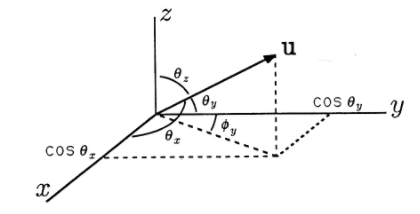
Consider the direction vector \(\mathrm{u}=\left\{\begin{array}{l}
\cos \theta_{x} \\
\cos \theta_{y} \\
\cos \theta_{z}
\end{array}\right\}\) as shown in Figure 5. What is the angle \(\psi_y\) between the projection of \(u\) into the \(x−y\) plane and the y-axis? This is important because it is R\(_z(\psi_y)\)that will put \(u\) in the \(y−z\) plane, and we need to know the angle \(\psi_y\) in order to carry out this rotation. First note that it is not the same as \(\theta_y\). From the geometry of the figure, we can write
\[\tan \varphi_{y}=\frac{\cos \theta_{x}}{\cos \theta_{y}} \nonumber \]
This gives us a formula for \(\psi_y\) in terms of the direction cosines of \(u\). With the two-argument arc tangent, we can write
\[\varphi_{y}=\tan ^{-1}\left(\cos \theta_{x}, \cos \theta_{y}\right) \nonumber \]
- Suppose point \(p'\) is in the \(y−z\) plane in three dimensions, \(p′=(0,y′,'',1)\). Find \(\theta\) so that R\(_x(\theta)\) will rotate \(p'\) to the positive z-axis. (Hint: Use the two-argument arc tangent. \(\theta\) will be a function of \(y'\) and \(z'\).)
- Let \(p\) be any point in three-dimensional space, \(p=(x,y,z,1)\). Find \(\psi\) so that R\(_z(\psi)\) rotates \(p\) into the \(y−z\) plane. (Hint: Sketch the situation in three-dimensions, then sketch a two-dimensional view looking down at the \(x−y\) plane from the positive z-axis. Compare with Example 2.) Your answers to parts (a) and (b) can be composed into an operator Z(p) that rotates a given point \(p\) to the positive z-axis, Z(p)=R\(_x(\theta)\)R\(_z(\psi)\).
- Let \(\mathscr{L}\) be a line in three-dimensional space specified by a point 1 = \((x,y,z,1)\) and the direction cosines \((\cos{\theta_x}, \cos{\theta_y}, \cos{\theta_z})\). Use the following procedure to derive a composite operator R\((\psi,\mathscr{L})\) that rotates by angle \(\psi\) about the line \(\mathscr{L}\):
- translate 1 to the origin;
- let u=\((\cos{\theta_x}, \cos{\theta_y}, \cos{\theta_z}, 1)\) and use Z(u) to align \(\mathscr{L}\) with the z-axis;
- rotate by \(\psi\) about the z-axis;
- undo step (ii); and
- undo step (i)