4.3: Programming Shared-Memory Multiprocessors

Introduction

In [Section 3.2], we examined the hardware used to implement shared-memory parallel processors and the software environment for a programmer who is using threads explicitly. In this chapter, we view these processors from a simpler vantage point. When programming these systems in FORTRAN, you have the advantage of the compiler’s support of these systems. At the top end of ease of use, we can simply add a flag or two on the compilation of our well-written code, set an environment variable, and voilá, we are executing in parallel. If you want some more control, you can add directives to particular loops where you know better than the compiler how the loop should be executed.¹ First we examine how well-written loops can benefit from automatic parallelism. Then we will look at the types of directives you can add to your program to assist the compiler in generating parallel code. While this chapter refers to running your code in parallel, most of the techniques apply to the vector-processor supercomputers as well.

Automatic Parallelization

So far in the book, we’ve covered the tough things you need to know to do parallel processing. At this point, assuming that your loops are clean, they use unit stride, and the iterations can all be done in parallel, all you have to do is turn on a compiler flag and buy a good parallel processor. For example, look at the following code:

      PARAMETER(NITER=300,N=1000000)
      REAL*8 A(N),X(N),B(N),C
      DO ITIME=1,NITER
        DO I=1,N
            A(I) = X(I) + B(I) * C
        ENDDO
        CALL WHATEVER(A,X,B,C)
      ENDDO

Here we have an iterative code that satisfies all the criteria for a good parallel loop. On a good parallel processor with a modern compiler, you are two flags away from executing in parallel. On Sun Solaris systems, the autopar flag turns on the automatic parallelization, and the loopinfo flag causes the compiler to describe the particular optimization performed for each loop. To compile this code under Solaris, you simply add these flags to your f77 call:

      E6000: f77 -O3 -autopar -loopinfo -o daxpy daxpy.f
      daxpy.f:
      "daxpy.f", line 6: not parallelized, call may be unsafe
      "daxpy.f", line 8: PARALLELIZED
      E6000: /bin/time daxpy

      real       30.9
      user       30.7
      sys         0.1
      E6000:

If you simply run the code, it’s executed using one thread. However, the code is enabled for parallel processing for those loops that can be executed in parallel. To execute the code in parallel, you need to set the UNIX environment to the number of parallel threads you wish to use to execute the code. On Solaris, this is done using the PARALLEL variable:

      E6000: setenv PARALLEL 1
      E6000: /bin/time daxpy

      real        30.9
      user        30.7
      sys          0.1
      E6000: setenv PARALLEL 2
      E6000: /bin/time daxpy

      real        15.6
      user        31.0
      sys          0.2
      E6000: setenv PARALLEL 4
      E6000: /bin/time daxpy

      real        8.2
      user       32.0
      sys         0.5
      E6000: setenv PARALLEL 8
      E6000: /bin/time daxpy

      real        4.3
      user       33.0
      sys         0.8

Speedup is the term used to capture how much faster the job runs using N processors compared to the performance on one processor. It is computed by dividing the single processor time by the multiprocessor time for each number of processors. [Figure 1] shows the wall time and speedup for this application.

Figure \(\PageIndex{1}\): Improving performance by adding processors

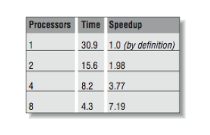
[Figure 2] shows this information graphically, plotting speedup versus the number of processors.

Figure \(\PageIndex{2}\): Ideal and actual performance improvement

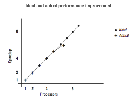
Note that for a while we get nearly perfect speedup, but we begin to see a measurable drop in speedup at four and eight processors. There are several causes for this. In all parallel applications, there is some portion of the code that can’t run in parallel. During those nonparallel times, the other processors are waiting for work and aren’t contributing to efficiency. This nonparallel code begins to affect the overall performance as more processors are added to the application.

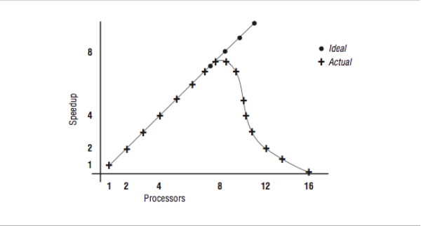
So you say, “this is more like it!” and immediately try to run with 12 and 16 threads. Now, we see the graph in [Figure 4] and the data from [Figure 3].

Figure \(\PageIndex{3}\): Increasing the number of threads

Figure \(\PageIndex{4}\): Diminishing returns

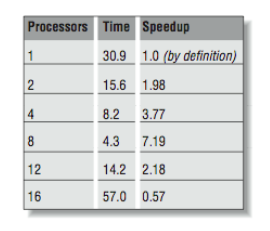
What has happened here? Things were going so well, and then they slowed down. We are running this program on a 16-processor system, and there are eight other active threads, as indicated below:

E6000:uptime
  4:00pm  up 19 day(s), 37 min(s), 5 users, load average: 8.00, 8.05, 8.14
E6000:

Once we pass eight threads, there are no available processors for our threads. So the threads must be time-shared between the processors, significantly slowing the overall operation. By the end, we are executing 16 threads on eight processors, and our performance is slower than with one thread. So it is important that you don’t create too many threads in these types of applications.

Compiler Considerations

Improving performance by turning on automatic parallelization is an example of the “smarter compiler” we discussed in earlier chapters. The addition of a single compiler flag has triggered a great deal of analysis on the part of the compiler including:

• Which loops can execute in parallel, producing the exact same results as the sequential executions of the loops? This is done by checking for dependencies that span iterations. A loop with no interiteration dependencies is called a DOALL loop.
• Which loops are worth executing in parallel? Generally very short loops gain no benefit and may execute more slowly when executing in parallel. As with loop unrolling, parallelism always has a cost. It is best used when the benefit far outweighs the cost.
• In a loop nest, which loop is the best candidate to be parallelized? Generally the best performance occurs when we parallelize the outermost loop of a loop nest. This way the overhead associated with beginning a parallel loop is amortized over a longer parallel loop duration.
• Can and should the loop nest be interchanged? The compiler may detect that the loops in a nest can be done in any order. One order may work very well for parallel code while giving poor memory performance. Another order may give unit stride but perform poorly with multiple threads. The compiler must analyze the cost/benefit of each approach and make the best choice.
• How do we break up the iterations among the threads executing a parallel loop? Are the iterations short with uniform duration, or long with wide variation of execution time? We will see that there are a number of different ways to accomplish this. When the programmer has given no guidance, the compiler must make an educated guess.

Even though it seems complicated, the compiler can do a surprisingly good job on a wide variety of codes. It is not magic, however. For example, in the following code we have a loop-carried flow dependency:

      PROGRAM DEP
      PARAMETER(NITER=300,N=1000000)
      REAL*4 A(N)

      DO ITIME=1,NITER
        CALL WHATEVER(A)
        DO I=2,N
            A(I) = A(I-1) + A(I) * C
        ENDDO
      ENDDO
      END

When we compile the code, the compiler gives us the following message:

      E6000: f77 -O3 -autopar -loopinfo -o dep dep.f
      dep.f:
      "dep.f", line 6: not parallelized, call may be unsafe
      "dep.f", line 8: not parallelized, unsafe dependence (a)
      E6000:

The compiler throws its hands up in despair, and lets you know that the loop at Line 8 had an unsafe dependence, and so it won’t automatically parallelize the loop. When the code is executed below, adding a thread does not affect the execution performance:

      E6000:setenv PARALLEL 1
      E6000:/bin/time dep

      real       18.1
      user       18.1
      sys         0.0
      E6000:setenv PARALLEL 2
      E6000:/bin/time dep

      real       18.3
      user       18.2
      sys         0.0
      E6000:

A typical application has many loops. Not all the loops are executed in parallel. It’s a good idea to run a profile of your application, and in the routines that use most of the CPU time, check to find out which loops are not being parallelized. Within a loop nest, the compiler generally chooses only one loop to execute in parallel.

Other Compiler Flags

In addition to the flags shown above, you may have other compiler flags available to you that apply across the entire program:

• You may have a compiler flag to enable the automatic parallelization of reduction operations. Because the order of additions can affect the final value when computing a sum of floating-point numbers, the compiler needs permission to parallelize summation loops.
• Flags that relax the compliance with IEEE floating-point rules may also give the compiler more flexibility when trying to parallelize a loop. However, you must be sure that it’s not causing accuracy problems in other areas of your code.
• Often a compiler has a flag called “unsafe optimization” or “assume no dependencies.” While this flag may indeed enhance the performance of an application with loops that have dependencies, it almost certainly produces incorrect results.

There is some value in experimenting with a compiler to see the particular combination that will yield good performance across a variety of applications. Then that set of compiler options can be used as a starting point when you encounter a new application.

Assisting the Compiler

If it were all that simple, you wouldn’t need this book. While compilers are extremely clever, there is still a lot of ways to improve the performance of your code without sacrificing its portability. Instead of converting the whole program to C and using a thread library, you can assist the compiler by adding compiler directives to our source code.

Compiler directives are typically inserted in the form of stylized FORTRAN comments. This is done so that a nonparallelizing compiler can ignore them and just look at the FORTRAN code, sans comments. This allows to you tune your code for parallel architectures without letting it run badly on a wide range of single-processor systems.

There are two categories of parallel-processing comments:

• Assertions
• Manual parallelization directives

Assertions tell the compiler certain things that you as the programmer know about the code that it might not guess by looking at the code. Through the assertions, you are attempting to assuage the compiler’s doubts about whether or not the loop is eligible for parallelization. When you use directives, you are taking full responsibility for the correct execution of the program. You are telling the compiler what to parallelize and how to do it. You take full responsibility for the output of the program. If the program produces meaningless results, you have no one to blame but yourself.

Assertions

In a previous example, we compiled a program and received the following output:

E6000: f77 -O3 -autopar -loopinfo -o dep dep.f
dep.f:
"dep.f", line 6: not parallelized, call may be unsafe
"dep.f", line 8: not parallelized, unsafe dependence (a)
E6000:

An uneducated programmer who has not read this book (or has not looked at the code) might exclaim, “What unsafe dependence, I never put one of those in my code!” and quickly add a no dependencies assertion. This is the essence of an assertion. Instead of telling the compiler to simply parallelize the loop, the programmer is telling the compiler that its conclusion that there is a dependence is incorrect. Usually the net result is that the compiler does indeed parallelize the loop.

We will briefly review the types of assertions that are typically supported by these compilers. An assertion is generally added to the code using a stylized comment.

No dependencies

A no dependencies or ignore dependencies directive tells the compiler that references don’t overlap. That is, it tells the compiler to generate code that may execute incorrectly if there are dependencies. You’re saying, “I know what I’m doing; it’s OK to overlap references.” A no dependencies directive might help the following loop:

DO I=1,N
  A(I) = A(I+K) * B(I)
ENDDO

If you know that k is greater than -1 or less than -n, you can get the compiler to parallelize the loop:

C$ASSERT NO_DEPENDENCIES
     DO I=1,N
       A(I) = A(I+K) * B(I)
     ENDDO

Of course, blindly telling the compiler that there are no dependencies is a prescription for disaster. If k equals -1, the example above becomes a recursive loop.

Relations

You will often see loops that contain some potential dependencies, making them bad candidates for a no dependencies directive. However, you may be able to supply some local facts about certain variables. This allows partial parallelization without compromising the results. In the code below, there are two potential dependencies because of subscripts involving k and j:

for (i=0; i<n; i++) {
    a[i] = a[i+k] * b[i];
    c[i] = c[i+j] * b[i];
}

Perhaps we know that there are no conflicts with references to a[i] and a[i+k]. But maybe we aren’t so sure about c[i] and c[i+j]. Therefore, we can’t say in general that there are no dependencies. However, we may be able to say something explicit about k (like “k is always greater than -1”), leaving j out of it. This information about the relationship of one expression to another is called a relation assertion. Applying a relation assertion allows the compiler to apply its optimization to the first statement in the loop, giving us partial parallelization.²

Again, if you supply inaccurate testimony that leads the compiler to make unsafe optimizations, your answer may be wrong.

Permutations

As we have seen elsewhere, when elements of an array are indirectly addressed, you have to worry about whether or not some of the subscripts may be repeated. In the code below, are the values of K(I) all unique? Or are there duplicates?

DO I=1,N
  A(K(I)) = A(K(I)) + B(I) * C
END DO

If you know there are no duplicates in K (i.e., that A(K(I)) is a permutation), you can inform the compiler so that iterations can execute in parallel. You supply the information using a permutation assertion.

No equivalences

Equivalenced arrays in FORTRAN programs provide another challenge for the compiler. If any elements of two equivalenced arrays appear in the same loop, most compilers assume that references could point to the same memory storage location and optimize very conservatively. This may be true even if it is abundantly apparent to you that there is no overlap whatsoever.

You inform the compiler that references to equivalenced arrays are safe with a no equivalences assertion. Of course, if you don’t use equivalences, this assertion has no effect.

Trip count

Each loop can be characterized by an average number of iterations. Some loops are never executed or go around just a few times. Others may go around hundreds of times:

C$ASSERT TRIPCOUNT>100
     DO I=L,N
       A(I) = B(I) + C(I)
     END DO

Your compiler is going to look at every loop as a candidate for unrolling or parallelization. It’s working in the dark, however, because it can’t tell which loops are important and tries to optimize them all. This can lead to the surprising experience of seeing your runtime go up after optimization!

A trip count assertion provides a clue to the compiler that helps it decide how much to unroll a loop or when to parallelize a loop.³ Loops that aren’t important can be identified with low or zero trip counts. Important loops have high trip counts.

Inline substitution

If your compiler supports procedure inlining, you can use directives and command-line switches to specify how many nested levels of procedures you would like to inline, thresholds for procedure size, etc. The vendor will have chosen reasonable defaults.

Assertions also let you choose subroutines that you think are good candidates for inlining. However, subject to its thresholds, the compiler may reject your choices. Inlining could expand the code so much that increased memory activity would claim back gains made by eliminating the procedure call. At higher optimization levels, the compiler is often capable of making its own choices for inlining candidates, provided it can find the source code for the routine under consideration.

Some compilers support a feature called interprocedural analysis. When this is done, the compiler looks across routine boundaries for its data flow analysis. It can perform significant optimizations across routine boundaries, including automatic inlining, constant propagation, and others.

No side effects

Without interprocedural analysis, when looking at a loop, if there is a subroutine call in the middle of the loop, the compiler has to treat the subroutine as if it will have the worst possible side effects. Also, it has to assume that there are dependencies that prevent the routine from executing simultaneously in two different threads.

Many routines (especially functions) don’t have any side effects and can execute quite nicely in separate threads because each thread has its own private call stack and local variables. If the routine is meaty, there will be a great deal of benefit in executing it in parallel.

Your computer may allow you to add a directive that tells you if successive sub-routine calls are independent:

C$ASSERT NO_SIDE_EFFECTS
     DO I=1,N
       CALL BIGSTUFF (A,B,C,I,J,K)
     END DO

Even if the compiler has all the source code, use of common variables or equivalences may mask call independence.

Manual Parallelism

At some point, you get tired of giving the compiler advice and hoping that it will reach the conclusion to parallelize your loop. At that point you move into the realm of manual parallelism. Luckily the programming model provided in FORTRAN insulates you from much of the details of exactly how multiple threads are managed at runtime. You generally control explicit parallelism by adding specially formatted comment lines to your source code. There are a wide variety of formats of these directives. In this section, we use the syntax that is part of the OpenMP standard. You generally find similar capabilities in each of the vendor compilers. The precise syntax varies slightly from vendor to vendor. (That alone is a good reason to have a standard.)

The basic programming model is that you are executing a section of code with either a single thread or multiple threads. The programmer adds a directive to summon additional threads at various points in the code. The most basic construct is called the parallel region.

Parallel regions

In a parallel region, the threads simply appear between two statements of straight-line code. A very trivial example might be the following using the OpenMP directive syntax:

        PROGRAM ONE
        EXTERNAL OMP_GET_THREAD_NUM, OMP_GET_MAX_THREADS
        INTEGER OMP_GET_THREAD_NUM, OMP_GET_MAX_THREADS
        IGLOB = OMP_GET_MAX_THREADS()
        PRINT *,’Hello There’
C$OMP PARALLEL PRIVATE(IAM), SHARED(IGLOB)
        IAM = OMP_GET_THREAD_NUM()
        PRINT *, ’I am ’, IAM, ’ of ’, IGLOB
C$OMP END PARALLEL
        PRINT *,’All Done’
        END

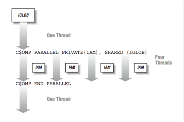
The C$OMP is the sentinel that indicates that this is a directive and not just another comment. The output of the program when run looks as follows:

    % setenv OMP_NUM_THREADS 4
    % a.out
    Hello There
    I am 0 of 4
    I am 3 of 4
    I am 1 of 4
    I am 2 of 4
    All Done
    %

Execution begins with a single thread. As the program encounters the PARALLEL directive, the other threads are activated to join the computation. So in a sense, as execution passes the first directive, one thread becomes four. Four threads execute the two statements between the directives. As the threads are executing independently, the order in which the print statements are displayed is somewhat random. The threads wait at the END PARALLEL directive until all threads have arrived. Once all threads have completed the parallel region, a single thread continues executing the remainder of the program.

In [Figure 5], the PRIVATE(IAM) indicates that the IAM variable is not shared across all the threads but instead, each thread has its own private version of the variable. The IGLOB variable is shared across all the threads. Any modification of IGLOB appears in all the other threads instantly, within the limitations of the cache coherency.

Figure \(\PageIndex{5}\): Data interactions during a parallel region

During the parallel region, the programmer typically divides the work among the threads. This pattern of going from single-threaded to multithreaded execution may be repeated many times throughout the execution of an application.

Because input and output are generally not thread-safe, to be completely correct, we should indicate that the print statement in the parallel section is only to be executed on one processor at any one time. We use a directive to indicate that this section of code is a critical section. A lock or other synchronization mechanism ensures that no more than one processor is executing the statements in the critical section at any one time:

C$OMP CRITICAL
        PRINT *, ’I am ’, IAM, ’ of ’, IGLOB
C$OMP END CRITICAL

Parallel loops

Quite often the areas of the code that are most valuable to execute in parallel are loops. Consider the following loop:

DO I=1,1000000
  TMP1 = ( A(I) ** 2 ) + ( B(I) ** 2 )
  TMP2 = SQRT(TMP1)
  B(I) = TMP2
ENDDO

To manually parallelize this loop, we insert a directive at the beginning of the loop:

C$OMP PARALLEL DO
      DO I=1,1000000
        TMP1 = ( A(I) ** 2 ) + ( B(I) ** 2 )
        TMP2 = SQRT(TMP1)
        B(I) = TMP2
      ENDDO
C$OMP END PARALLEL DO

When this statement is encountered at runtime, the single thread again summons the other threads to join the computation. However, before the threads can start working on the loop, there are a few details that must be handled. The PARALLEL DO directive accepts the data classification and scoping clauses as in the parallel section directive earlier. We must indicate which variables are shared across all threads and which variables have a separate copy in each thread. It would be a disaster to have TMP1 and TMP2 shared across threads. As one thread takes the square root of TMP1, another thread would be resetting the contents of TMP1. A(I) and B(I) come from outside the loop, so they must be shared. We need to augment the directive as follows:

C$OMP PARALLEL DO SHARED(A,B) PRIVATE(I,TMP1,TMP2)
      DO I=1,1000000
        TMP1 = ( A(I) ** 2 ) + ( B(I) ** 2 )
        TMP2 = SQRT(TMP1)
        B(I) = TMP2
      ENDDO
C$OMP END PARALLEL DO

The iteration variable I also must be a thread-private variable. As the different threads increment their way through their particular subset of the arrays, they don’t want to be modifying a global value for I.

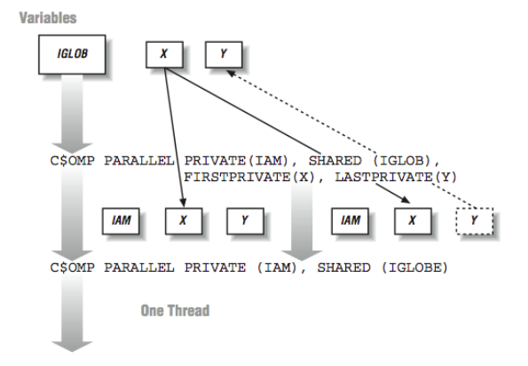
There are a number of other options as to how data will be operated on across the threads. This summarizes some of the other data semantics available:

• Firstprivate: These are thread-private variables that take an initial value from the global variable of the same name immediately before the loop begins executing.
• Lastprivate: These are thread-private variables except that the thread that executes the last iteration of the loop copies its value back into the global variable of the same name.
• Reduction: This indicates that a variable participates in a reduction operation that can be safely done in parallel. This is done by forming a partial reduction using a local variable in each thread and then combining the partial results at the end of the loop.

Each vendor may have different terms to indicate these data semantics, but most support all of these common semantics. [Figure 6] shows how the different types of data semantics operate.

Now that we have the data environment set up for the loop, the only remaining problem that must be solved is which threads will perform which iterations. It turns out that this is not a trivial task, and a wrong choice can have a significant negative impact on our overall performance.

Iteration scheduling

There are two basic techniques (along with a few variations) for dividing the iterations in a loop between threads. We can look at two extreme examples to get an idea of how this works:

C VECTOR ADD
      DO IPROB=1,10000
         A(IPROB) = B(IPROB) + C(IPROB)
      ENDDO

C PARTICLE TRACKING
       DO IPROB=1,10000
          RANVAL = RAND(IPROB)
          CALL ITERATE_ENERGY(RANVAL) ENDDO
       ENDDO

Figure \(\PageIndex{6}\): Variables during a parallel region

In both loops, all the computations are independent, so if there were 10,000 processors, each processor could execute a single iteration. In the vector-add example, each iteration would be relatively short, and the execution time would be relatively constant from iteration to iteration. In the particle tracking example, each iteration chooses a random number for an initial particle position and iterates to find the minimum energy. Each iteration takes a relatively long time to complete, and there will be a wide variation of completion times from iteration to iteration.

These two examples are effectively the ends of a continuous spectrum of the iteration scheduling challenges facing the FORTRAN parallel runtime environment:

Static

At the beginning of a parallel loop, each thread takes a fixed continuous portion of iterations of the loop based on the number of threads executing the loop.

Dynamic

With dynamic scheduling, each thread processes a chunk of data and when it has completed processing, a new chunk is processed. The chunk size can be varied by the programmer, but is fixed for the duration of the loop.

These two example loops can show how these iteration scheduling approaches might operate when executing with four threads. In the vector-add loop, static scheduling would distribute iterations 1–2500 to Thread 0, 2501–5000 to Thread 1, 5001–7500 to Thread 2, and 7501–10000 to Thread 3. In [Figure 7], the mapping of iterations to threads is shown for the static scheduling option.

Figure \(\PageIndex{7}\): Iteration assignment for static scheduling

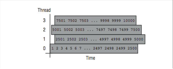
Since the loop body (a single statement) is short with a consistent execution time, static scheduling should result in roughly the same amount of overall work (and time if you assume a dedicated CPU for each thread) assigned to each thread per loop execution.

An advantage of static scheduling may occur if the entire loop is executed repeatedly. If the same iterations are assigned to the same threads that happen to be running on the same processors, the cache might actually contain the values for A, B, and C from the previous loop execution.⁴ The runtime pseudo-code for static scheduling in the first loop might look as follows:

C VECTOR ADD - Static Scheduled
     ISTART = (THREAD_NUMBER * 2500 ) + 1
     IEND = ISTART + 2499
     DO ILOCAL = ISTART,IEND
       A(ILOCAL) = B(ILOCAL) + C(ILOCAL)
     ENDDO

It’s not always a good strategy to use the static approach of giving a fixed number of iterations to each thread. If this is used in the second loop example, long and varying iteration times would result in poor load balancing. A better approach is to have each processor simply get the next value for IPROB each time at the top of the loop.

That approach is called dynamic scheduling, and it can adapt to widely varying iteration times. In [Figure 8], the mapping of iterations to processors using dynamic scheduling is shown. As soon as a processor finishes one iteration, it processes the next available iteration in order.

Figure \(\PageIndex{8}\): Iteration assignment in dynamic scheduling

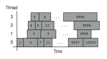
If a loop is executed repeatedly, the assignment of iterations to threads may vary due to subtle timing issues that affect threads. The pseudo-code for the dynamic scheduled loop at runtime is as follows:

C PARTICLE TRACKING - Dynamic Scheduled
     IPROB = 0
     WHILE (IPROB <= 10000 )
       BEGIN_CRITICAL_SECTION
         IPROB = IPROB + 1
         ILOCAL = IPROB
       END_CRITICAL_SECTION
       RANVAL = RAND(ILOCAL)
       CALL ITERATE_ENERGY(RANVAL)
     ENDWHILE

ILOCAL is used so that each thread knows which iteration is currently processing. The IPROB value is altered by the next thread executing the critical section.

While the dynamic iteration scheduling approach works well for this particular loop, there is a significant negative performance impact if the programmer were to use the wrong approach for a loop. For example, if the dynamic approach were used for the vector-add loop, the time to process the critical section to determine which iteration to process may be larger than the time to actually process the iteration. Furthermore, any cache affinity of the data would be effectively lost because of the virtually random assignment of iterations to processors.

In between these two approaches are a wide variety of techniques that operate on a chunk of iterations. In some techniques the chunk size is fixed, and in others it varies during the execution of the loop. In this approach, a chunk of iterations are grabbed each time the critical section is executed. This reduces the scheduling overhead, but can have problems in producing a balanced execution time for each processor. The runtime is modified as follows to perform the particle tracking loop example using a chunk size of 100:

      IPROB = 1
      CHUNKSIZE = 100
      WHILE (IPROB <= 10000 )
        BEGIN_CRITICAL_SECTION
          ISTART = IPROB
          IPROB = IPROB + CHUNKSIZE
        END_CRITICAL_SECTION
        DO ILOCAL = ISTART,ISTART+CHUNKSIZE-1
          RANVAL = RAND(ILOCAL)
          CALL ITERATE_ENERGY(RANVAL)
        ENDDO
      ENDWHILE

The choice of chunk size is a compromise between overhead and termination imbalance. Typically the programmer must get involved through directives in order to control chunk size.

Part of the challenge of iteration distribution is to balance the cost (or existence) of the critical section against the amount of work done per invocation of the critical section. In the ideal world, the critical section would be free, and all scheduling would be done dynamically. Parallel/vector supercomputers with hardware assistance for load balancing can nearly achieve the ideal using dynamic approaches with relatively small chunk size.

Because the choice of loop iteration approach is so important, the compiler relies on directives from the programmer to specify which approach to use. The following example shows how we can request the proper iteration scheduling for our loops:

C VECTOR ADD
C$OMP PARALLEL DO PRIVATE(IPROB) SHARED(A,B,C) SCHEDULE(STATIC)
      DO IPROB=1,10000
         A(IPROB) = B(IPROB) + C(IPROB)
      ENDDO
C$OMP END PARALLEL DO
C PARTICLE TRACKING
C$OMP PARALLEL DO PRIVATE(IPROB,RANVAL) SCHEDULE(DYNAMIC)
      DO IPROB=1,10000
         RANVAL = RAND(IPROB)
         CALL ITERATE_ENERGY(RANVAL)
      ENDDO
C$OMP END PARALLEL DO

Closing Notes

Using data flow analysis and other techniques, modern compilers can peer through the clutter that we programmers innocently put into our code and see the patterns of the actual computations. In the field of high performance computing, having great parallel hardware and a lousy automatic parallelizing compiler generally results in no sales. Too many of the benchmark rules allow only a few compiler options to be set.

Physicists and chemists are interested in physics and chemistry, not computer science. If it takes 1 hour to execute a chemistry code without modifications and after six weeks of modifications the same code executes in 20 minutes, which is better? Well from a chemist’s point of view, one took an hour, and the other took 1008 hours and 20 minutes, so the answer is obvious.⁵ Although if the program were going to be executed thousands of times, the tuning might be a win for the programmer. The answer is even more obvious if it again takes six weeks to tune the program every time you make a modification to the program.

In some ways, assertions have become less popular than directives. This is due to two factors: (1) compilers are getting better at detecting parallelism even if they have to rewrite some code to do so, and (2) there are two kinds of programmers: those who know exactly how to parallelize their codes and those who turn on the “safe” auto-parallelize flags on their codes. Assertions fall in the middle ground, somewhere between where the programmer does not want to control all the details but kind of feels that the loop can be parallelized.

You can get online documentation of the OpenMP syntax used in these examples at www.openmp.org.

Exercises

Exercise \(\PageIndex{1}\)

Take a static, highly parallel program with a relative large inner loop. Compile the application for parallel execution. Execute the application increasing the threads. Examine the behavior when the number of threads exceed the available processors. See if different iteration scheduling approaches make a difference.

Exercise \(\PageIndex{2}\)

Take the following loop and execute with several different iteration scheduling choices. For chunk-based scheduling, use a large chunk size, perhaps 100,000. See if any approach performs better than static scheduling:

      DO I=1,4000000
        A(I) = B(I) * 2.34
      ENDDO

Exercise \(\PageIndex{3}\)

Execute the following loop for a range of values for N from 1 to 16 million:

      DO I=1,N
        A(I) = B(I) * 2.34
      ENDDO

Run the loop in a single processor. Then force the loop to run in parallel. At what point do you get better performance on multiple processors? Do the number of threads affect your observations?

Exercise \(\PageIndex{4}\)

Use an explicit parallelization directive to execute the following loop in parallel with a chunk size of 1:

      J = 0
C$OMP PARALLEL DO PRIVATE(I) SHARED(J) SCHEDULE(DYNAMIC)
      DO I=1,1000000
       J = J + 1
      ENDDO
      PRINT *, J
C$OMP END PARALLEL DO

Execute the loop with a varying number of threads, including one. Also compile and execute the code in serial. Compare the output and execution times. What do the results tell you about cache coherency? About the cost of moving data from one cache to another, and about critical section costs

---

Footnotes

1. If you have skipped all the other chapters in the book and jumped to this one, don’t be surprised if some of the terminology is unfamiliar. While all those chapters seemed to contain endless boring detail, they did contain some basic terminology. So those of us who read all those chapters have some common terminology needed for this chapter. If you don’t go back and read all the chapters, don’t complain about the big words we keep using in this chapter!
2. Notice that, if you were tuning by hand, you could split this loop into two: one parallelizable and one not.
3. The assertion is made either by hand or from a profiler.
4. The operating system and runtime library actually go to some lengths to try to make this happen. This is another reason not to have more threads than available processors, which causes unnecessary context switching.
5. On the other hand, if the person is a computer scientist, improving the performance might result in anything from a poster session at a conference to a journal article! This makes for lots of intra-departmental masters degree projects.