1.2: Perceptrons

What is a neural network? To get started, I'll explain a type of artificial neuron called a perceptron. Perceptrons were developed in the 1950s and 1960s by the scientist Frank Rosenblatt, inspired by earlier work by Warren McCulloch and Walter Pitts. Today, it's more common to use other models of artificial neurons - in this book, and in much modern work on neural networks, the main neuron model used is one called the sigmoid neuron. We'll get to sigmoid neurons shortly. But to understand why sigmoid neurons are defined the way they are, it's worth taking the time to first understand perceptrons.

So how do perceptrons work? A perceptron takes several binary inputs, \(x_1,x_2,…\) and produces a single binary output:

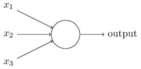
In the example shown the perceptron has three inputs, \(x_1,x_2,x_3\) In general it could have more or fewer inputs. Rosenblatt proposed a simple rule to compute the output. He introduced weights, \(w_1,w_2,…\) real numbers expressing the importance of the respective inputs to the output. The neuron's output, \(0\) or \(1\), is determined by whether the weighted sum \(\sum_{j} w_jx_j\) is less than or greater than some threshold value. Just like the weights, the threshold is a real number which is a parameter of the neuron. To put it in more precise algebraic terms:

\[output= \begin{cases} 0 & \text{if} \sum_{j} w_jx_j\le \text{threshold} \\ 1 & \text{if} \sum_{j} w_jx_j\gt \text{threshold} \end{cases}\]

That's all there is to how a perceptron works!

That's the basic mathematical model. A way you can think about the perceptron is that it's a device that makes decisions by weighing up evidence. Let me give an example. It's not a very realistic example, but it's easy to understand, and we'll soon get to more realistic examples. Suppose the weekend is coming up, and you've heard that there's going to be a cheese festival in your city. You like cheese, and are trying to decide whether or not to go to the festival. You might make your decision by weighing up three factors:

1. Is the weather good?
2. Does your boyfriend or girlfriend want to accompany you?
3. Is the festival near public transit? (You don't own a car).

We can represent these three factors by corresponding binary variables \(x_1,x_2 and x_3.\) For instance, we'd have \(x_1=1\) if the weather is good, and \(x_1=0\) if the weather is bad. Similarly, \(x_2=1\) if your boyfriend or girlfriend wants to go, and \(x_2=0\) if not. And similarly again for \(x_3\) and public transit.

Now, suppose you absolutely adore cheese, so much so that you're happy to go to the festival even if your boyfriend or girlfriend is uninterested and the festival is hard to get to. But perhaps you really loathe bad weather, and there's no way you'd go to the festival if the weather is bad. You can use perceptrons to model this kind of decision-making. One way to do this is to choose a weight \(w_1=6\) for the weather, and \(w_2=2\) and \(w_3=2\) for the other conditions. The larger value of \(w_1\) indicates that the weather matters a lot to you, much more than whether your boyfriend or girlfriend joins you, or the nearness of public transit. Finally, suppose you choose a threshold of \(5\) for the perceptron. With these choices, the perceptron implements the desired decision-making model, outputting \(1\) whenever the weather is good, and \(0\) whenever the weather is bad. It makes no difference to the output whether your boyfriend or girlfriend wants to go, or whether public transit is nearby.

By varying the weights and the threshold, we can get different models of decision-making. For example, suppose we instead chose a threshold of \(3\). Then the perceptron would decide that you should go to the festival whenever the weather was good or when both the festival was near public transit and your boyfriend or girlfriend was willing to join you. In other words, it'd be a different model of decision-making. Dropping the threshold means you're more willing to go to the festival.

Obviously, the perceptron isn't a complete model of human decision-making! But what the example illustrates is how a perceptron can weigh up different kinds of evidence in order to make decisions. And it should seem plausible that a complex network of perceptrons could make quite subtle decisions:

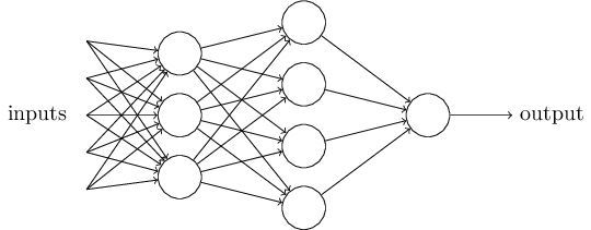
In this network, the first column of perceptrons - what we'll call the first layer of perceptrons - is making three very simple decisions, by weighing the input evidence. What about the perceptrons in the second layer? Each of those perceptrons is making a decision by weighing up the results from the first layer of decision-making. In this way a perceptron in the second layer can make a decision at a more complex and more abstract level than perceptrons in the first layer. And even more complex decisions can be made by the perceptron in the third layer. In this way, a many-layer network of perceptrons can engage in sophisticated decision making.

Incidentally, when I defined perceptrons I said that a perceptron has just a single output. In the network above the perceptrons look like they have multiple outputs. In fact, they're still single output. The multiple output arrows are merely a useful way of indicating that the output from a perceptron is being used as the input to several other perceptrons. It's less unwieldy than drawing a single output line which then splits.

Let's simplify the way we describe perceptrons. The condition \(\sum_{j} w_jx_j\gt \text{threshold}\) is cumbersome, and we can make two notational changes to simplify it. The first change is to write \(\sum_{j} w_jx_j\) as a dot product, \(w⋅x ≡ \sum_{j} w_jx_j\) where \(w\) and \(x\) are vectors whose components are the weights and inputs, respectively. The second change is to move the threshold to the other side of the inequality, and to replace it by what's known as the perceptron's bias, \(b ≡ −threshold\). Using the bias instead of the threshold, the perceptron rule can be rewritten:

\[output= \begin{cases} 0 & \text{if \(w.x + b\)} \le 0 \\ 1 & \text{if \(w.x + b\)} \gt 0 \end{cases}\]

You can think of the bias as a measure of how easy it is to get the perceptron to output a \(1\). Or to put it in more biological terms, the bias is a measure of how easy it is to get the perceptron to fire. For a perceptron with a really big bias, it's extremely easy for the perceptron to output a \(1\). But if the bias is very negative, then it's difficult for the perceptron to output a \(1\). Obviously, introducing the bias is only a small change in how we describe perceptrons, but we'll see later that it leads to further notational simplifications. Because of this, in the remainder of the book we won't use the threshold, we'll always use the bias.

I've described perceptrons as a method for weighing evidence to make decisions. Another way perceptrons can be used is to compute the elementary logical functions we usually think of as underlying computation, functions such as AND, OR , and NAND. For example, suppose we have a perceptron with two inputs, each with weight \(−2\), and an overall bias of \(3\). Here's our perceptron:

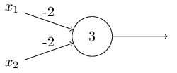
Then we see that input \(00\) produces output \(1\), since \((−2)∗0 + (−2)∗0 +3 = 3\) is positive. Here, I've introduced the \(∗\) symbol to make the multiplications explicit. Similar calculations show that the inputs \(01\) and \(10\) produce output \(11\). But the input \(11\) produces output \(0\), since \( (−2)∗1 + (−2)∗1 +3 = −1 \) is negative. And so our perceptron implements a NAND gate!

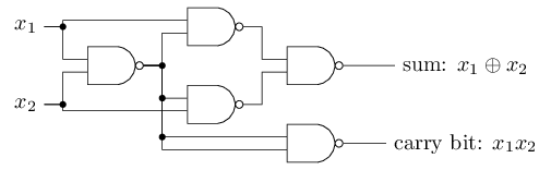
The NAND example shows that we can use perceptrons to compute simple logical functions. In fact, we can use networks of perceptrons to compute any logical function at all. The reason is that the NAND gate is universal for computation, that is, we can build any computation up out of NAND gates. For example, we can use NAND gates to build a circuit which adds two bits, \(x_1\) and \(x_2\). This requires computing the bitwise sum, \(x_1⊕x_2\), as well as a carry bit which is set to \(1\) when both \(x_1\) and \(x_2\) are \(1\), i.e., the carry bit is just the bitwise product \(x_1x_2\) :

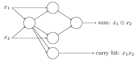
To get an equivalent network of perceptrons we replace all the NAND gates by perceptrons with two inputs, each with weight \(−2\), and an overall bias of \(3\). Here's the resulting network. Note that I've moved the perceptron corresponding to the bottom right NAND gate a little, just to make it easier to draw the arrows on the diagram:

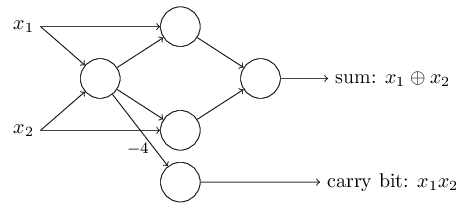
One notable aspect of this network of perceptrons is that the output from the leftmost perceptron is used twice as input to the bottommost perceptron. When I defined the perceptron model I didn't say whether this kind of double-output-to-the-same-place was allowed. Actually, it doesn't much matter. If we don't want to allow this kind of thing, then it's possible to simply merge the two lines, into a single connection with a weight of \(-4\) instead of two connections with \(-2\) weights. (If you don't find this obvious, you should stop and prove to yourself that this is equivalent.) With that change, the network looks as follows, with all unmarked weights equal to \(-2\), all biases equal to \(3\), and a single weight of \(-4\), as marked:

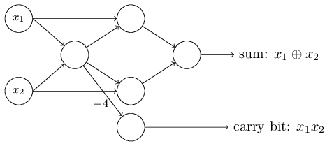
Up to now I've been drawing inputs like \(x_1\) and \(x_2\) as variables floating to the left of the network of perceptrons. In fact, it's conventional to draw an extra layer of perceptrons - the input layer- to encode the inputs:

This notation for input perceptrons, in which we have an output, but no inputs,

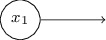
is a shorthand. It doesn't actually mean a perceptron with no inputs. To see this, suppose we did have a perceptron with no inputs. Then the weighted sum \(\sum_{j} w_jx_j\) would always be zero, and so the perceptron would output \(1\) if \(b\gt 0\), and \(0\) if \(b\le 0\). That is, the perceptron would simply output a fixed value, not the desired value (\(x_1\), in the example above). It's better to think of the input perceptrons as not really being perceptrons at all, but rather special units which are simply defined to output the desired values, \(x_1,x_2,…\)

The adder example demonstrates how a network of perceptrons can be used to simulate a circuit containing many NAND gates. And because NAND gates are universal for computation, it follows that perceptrons are also universal for computation.

The computational universality of perceptrons is simultaneously reassuring and disappointing. It's reassuring because it tells us that networks of perceptrons can be as powerful as any other computing device. But it's also disappointing, because it makes it seem as though perceptrons are merely a new type of NAND gate. That's hardly big news!

However, the situation is better than this view suggests. It turns out that we can devise learning algorithms which can automatically tune the weights and biases of a network of artificial neurons. This tuning happens in response to external stimuli, without direct intervention by a programmer. These learning algorithms enable us to use artificial neurons in a way which is radically different to conventional logic gates. Instead of explicitly laying out a circuit of NAND and other gates, our neural networks can simply learn to solve problems, sometimes problems where it would be extremely difficult to directly design a conventional circuit.