4.5: Fixing up the step functions

Up to now, we've been assuming that our neurons can produce step functions exactly. That's a pretty good approximation, but it is only an approximation. In fact, there will be a narrow window of failure, illustrated in the following graph, in which the function behaves very differently from a step function:

In these windows of failure the explanation I've given for universality will fail.

Now, it's not a terrible failure. By making the weights input to the neurons big enough we can make these windows of failure as small as we like. Certainly, we can make the window much narrower than I've shown above - narrower, indeed, than our eye could see. So perhaps we might not worry too much about this problem.

Nonetheless, it'd be nice to have some way of addressing the problem.

In fact, the problem turns out to be easy to fix. Let's look at the fix for neural networks computing functions with just one input and one output. The same ideas work also to address the problem when there are more inputs and outputs.

In particular, suppose we want our network to compute some function, ff. As before, we do this by trying to design our network so that the weighted output from our hidden layer of neurons is \(σ^−1∘f(x)\):

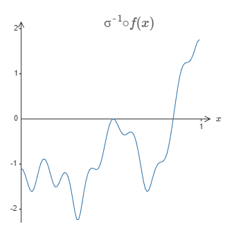
If we were to do this using the technique described earlier, we'd use the hidden neurons to produce a sequence of bump functions:

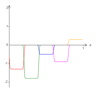
Again, I've exaggerated the size of the windows of failure, in order to make them easier to see. It should be pretty clear that if we add all these bump functions up we'll end up with a reasonable approximation to \(σ^−1∘f(x)\), except within the windows of failure.

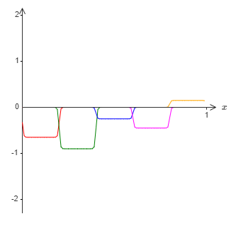
Suppose that instead of using the approximation just described, we use a set of hidden neurons to compute an approximation to half our original goal function, i.e., to \(σ^−1∘f(x)/2\). Of course, this looks just like a scaled down version of the last graph:

And suppose we use another set of hidden neurons to compute an approximation to \(σ^−1∘f(x)/2\), but with the bases of the bumps shifted by half the width of a bump:

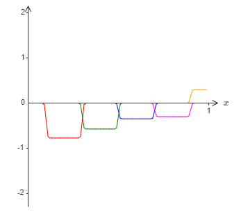
Now we have two different approximations to \(σ^−1∘f(x)/2\). If we add up the two approximations we'll get an overall approximation to \(σ^−1∘f(x)\). That overall approximation will still have failures in small windows. But the problem will be much less than before. The reason is that points in a failure window for one approximation won't be in a failure window for the other. And so the approximation will be a factor roughly \(2\) better in those windows.

We could do even better by adding up a large number, \(M\), of overlapping approximations to the function \(σ^−1∘f(x)/M\). Provided the windows of failure are narrow enough, a point will only ever be in one window of failure. And provided we're using a large enough number \(M\) of overlapping approximations, the result will be an excellent overall approximation.

Conclusion

The explanation for universality we've discussed is certainly not a practical prescription for how to compute using neural networks! In this, it's much like proofs of universality for NAND gates and the like. For this reason, I've focused mostly on trying to make the construction clear and easy to follow, and not on optimizing the details of the construction. However, you may find it a fun and instructive exercise to see if you can improve the construction.

Although the result isn't directly useful in constructing networks, it's important because it takes off the table the question of whether any particular function is computable using a neural network. The answer to that question is always "yes". So the right question to ask is not whether any particular function is computable, but rather what's a good way to compute the function.

The universality construction we've developed uses just two hidden layers to compute an arbitrary function. Furthermore, as we've discussed, it's possible to get the same result with just a single hidden layer. Given this, you might wonder why we would ever be interested in deep networks, i.e., networks with many hidden layers. Can't we simply replace those networks with shallow, single hidden layer networks?

Chapter acknowledgments: Thanks to Jen Dodd and Chris Olah for many discussions about universality in neural networks. My thanks, in particular, to Chris for suggesting the use of a lookup table to prove universality. The interactive visual form of the chapter is inspired by the work of people such as Mike Bostock, Amit Patel, Bret Victor, and Steven Wittens.

While in principle that's possible, there are good practical reasons to use deep networks. As argued in Chapter 1, deep networks have a hierarchical structure which makes them particularly well adapted to learn the hierarchies of knowledge that seem to be useful in solving real-world problems. Put more concretely, when attacking problems such as image recognition, it helps to use a system that understands not just individual pixels, but also increasingly more complex concepts: from edges to simple geometric shapes, all the way up through complex, multi-object scenes. In later chapters, we'll see evidence suggesting that deep networks do a better job than shallow networks at learning such hierarchies of knowledge. To sum up: universality tells us that neural networks can compute any function; and empirical evidence suggests that deep networks are the networks best adapted to learn the functions useful in solving many real-world problems.