
7.2: Treap - A Randomized Binary Search Tree
- Page ID
- 8466

The problem with random binary search trees is, of course, that they are not dynamic. They don't support the \(\mathtt{add(x)}\) or \(\mathtt{remove(x)}\) operations needed to implement the SSet interface. In this section we describe a data structure called a Treap that uses Lemma 7.1.1 to implement the SSet interface.2
A node in a Treap is like a node in a BinarySearchTree in that it has a data value, \(\mathtt{x}\), but it also contains a unique numerical priority, \(\mathtt{p}\), that is assigned at random:
    class Node<T> extends BinarySearchTree.BSTNode<Node<T>,T> {
        int p;
    }
In addition to being a binary search tree, the nodes in a Treap also obey the heap property:
- (Heap Property) At every node \(\mathtt{u}\), except the root, \(\texttt{u.parent.p} < \texttt{u.p}\).
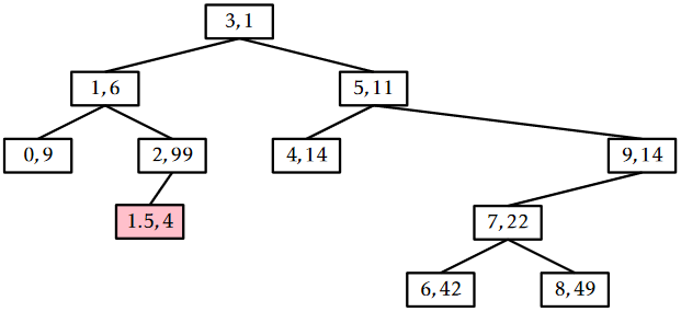
In other words, each node has a priority smaller than that of its two children. An example is shown in Figure \(\PageIndex{1}\).

The heap and binary search tree conditions together ensure that, once the key (\(\mathtt{x}\)) and priority (\(\mathtt{p}\)) for each node are defined, the shape of the Treap is completely determined. The heap property tells us that the node with minimum priority has to be the root, \(\mathtt{r}\), of the Treap. The binary search tree property tells us that all nodes with keys smaller than \(\texttt{r.x}\) are stored in the subtree rooted at \(\texttt{r.left}\) and all nodes with keys larger than \(\texttt{r.x}\) are stored in the subtree rooted at \(\texttt{r.right}\).
The important point about the priority values in a Treap is that they are unique and assigned at random. Because of this, there are two equivalent ways we can think about a Treap. As defined above, a Treap obeys the heap and binary search tree properties. Alternatively, we can think of a Treap as a BinarySearchTree whose nodes were added in increasing order of priority. For example, the Treap in Figure \(\PageIndex{1}\) can be obtained by adding the sequence of \((\mathtt{x},\mathtt{p})\) values
\[ \langle (3,1), (1,6), (0,9), (5,11), (4,14), (9,17), (7,22), (6,42), (8,49), (2,99) \rangle \nonumber\]
into a BinarySearchTree.
Since the priorities are chosen randomly, this is equivalent to taking a random permutation of the keys--in this case the permutation is
\[ \langle 3, 1, 0, 5, 9, 4, 7, 6, 8, 2 \rangle \nonumber\]
--and adding these to a BinarySearchTree. But this means that the shape of a treap is identical to that of a random binary search tree. In particular, if we replace each key \(\mathtt{x}\) by its rank,3 then Lemma 7.1.1 applies. Restating Lemma 7.1.1 in terms of Treaps, we have:
In a Treap that stores a set \(S\) of \(\mathtt{n}\) keys, the following statements hold:
- For any \(\mathtt{x}\in S\), the expected length of the search path for \(\mathtt{x}\) is \(H_{r(\mathtt{x})+1} + H_{\mathtt{n}-r(\mathtt{x})} - O(1)\).
- For any \(\mathtt{x}\not\in S\), the expected length of the search path for \(\mathtt{x}\) is \(H_{r(\mathtt{x})} + H_{\mathtt{n}-r(\mathtt{x})}\).
Here, \(r(\mathtt{x})\) denotes the rank of \(\mathtt{x}\) in the set \(S\cup\{\mathtt{x}\}\).
Again, we emphasize that the expectation in Lemma \(\PageIndex{1}\) is taken over the random choices of the priorities for each node. It does not require any assumptions about the randomness in the keys.
Lemma \(\PageIndex{1}\) tells us that Treaps can implement the \(\mathtt{find(x)}\) operation efficiently. However, the real benefit of a Treap is that it can support the \(\mathtt{add(x)}\) and \(\mathtt{delete(x)}\) operations. To do this, it needs to perform rotations in order to maintain the heap property. Refer to Figure \(\PageIndex{2}\). A rotation in a binary search tree is a local modification that takes a parent \(\mathtt{u}\) of a node \(\mathtt{w}\) and makes \(\mathtt{w}\) the parent of \(\mathtt{u}\), while preserving the binary search tree property. Rotations come in two flavours: left or right depending on whether \(\mathtt{w}\) is a right or left child of \(\mathtt{u}\), respectively.
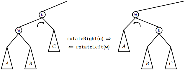
The code that implements this has to handle these two possibilities and be careful of a boundary case (when \(\mathtt{u}\) is the root), so the actual code is a little longer than Figure \(\PageIndex{2}\) would lead a reader to believe:
    void rotateLeft(Node u) {
        Node w = u.right;
        w.parent = u.parent;
        if (w.parent != nil) {
            if (w.parent.left == u) {
                w.parent.left = w;
            } else {
                w.parent.right = w;
            }
        }
        u.right = w.left;
        if (u.right != nil) {
            u.right.parent = u;
        }
        u.parent = w;
        w.left = u;
        if (u == r) { r = w; r.parent = nil; }
    }
    void rotateRight(Node u) {
        Node w = u.left;
        w.parent = u.parent;
        if (w.parent != nil) {
            if (w.parent.left == u) {
                w.parent.left = w;
            } else {
                w.parent.right = w;
            }
        }
        u.left = w.right;
        if (u.left != nil) {
            u.left.parent = u;
        }
        u.parent = w;
        w.right = u;
        if (u == r) { r = w; r.parent = nil; }
    }
In terms of the Treap data structure, the most important property of a rotation is that the depth of \(\mathtt{w}\) decreases by one while the depth of \(\mathtt{u}\) increases by one.
Using rotations, we can implement the \(\mathtt{add(x)}\) operation as follows: We create a new node, \(\mathtt{u}\), assign \(\mathtt{u\texttt{.}x=x}\), and pick a random value for \(\texttt{u.p}\). Next we add \(\mathtt{u}\) using the usual \(\mathtt{add(x)}\) algorithm for a BinarySearchTree, so that \(\mathtt{u}\) is now a leaf of the Treap. At this point, our Treap satisfies the binary search tree property, but not necessarily the heap property. In particular, it may be the case that \(\mathtt{u.parent.p > u.p}\). If this is the case, then we perform a rotation at node \(\mathtt{w}\)= \(\texttt{u.parent}\) so that \(\mathtt{u}\) becomes the parent of \(\mathtt{w}\). If \(\mathtt{u}\) continues to violate the heap property, we will have to repeat this, decreasing \(\mathtt{u}\)'s depth by one every time, until \(\mathtt{u}\) either becomes the root or \(\texttt{u.parent.p} < \texttt{u.p}\).
    boolean add(T x) {
        Node<T> u = newNode();
        u.x = x;
        u.p = rand.nextInt();
        if (super.add(u)) {
            bubbleUp(u);
            return true;
        }
        return false;
    }
    void bubbleUp(Node<T> u) {
        while (u.parent != nil && u.parent.p > u.p) {
            if (u.parent.right == u) {
                rotateLeft(u.parent);
            } else {
                rotateRight(u.parent);
            }
        }
        if (u.parent == nil) {
            r = u;
        }
    }
An example of an \(\mathtt{add(x)}\) operation is shown in Figure \(\PageIndex{3}\).
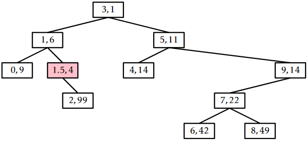
The running time of the \(\mathtt{add(x)}\) operation is given by the time it takes to follow the search path for \(\mathtt{x}\) plus the number of rotations performed to move the newly-added node, \(\mathtt{u}\), up to its correct location in the Treap. By Lemma \(\PageIndex{1}\), the expected length of the search path is at most \(2\ln \mathtt{n}+O(1)\). Furthermore, each rotation decreases the depth of \(\mathtt{u}\). This stops if \(\mathtt{u}\) becomes the root, so the expected number of rotations cannot exceed the expected length of the search path. Therefore, the expected running time of the \(\mathtt{add(x)}\) operation in a Treap is \(O(\log \mathtt{n})\). (Exercise 7.3.5 asks you to show that the expected number of rotations performed during an addition is actually only \(O(1)\).)
The \(\mathtt{remove(x)}\) operation in a Treap is the opposite of the \(\mathtt{add(x)}\) operation. We search for the node, \(\mathtt{u}\), containing \(\mathtt{x}\), then perform rotations to move \(\mathtt{u}\) downwards until it becomes a leaf, and then we splice \(\mathtt{u}\) from the Treap. Notice that, to move \(\mathtt{u}\) downwards, we can perform either a left or right rotation at \(\mathtt{u}\), which will replace \(\mathtt{u}\) with \(\texttt{u.right}\) or \(\texttt{u.left}\), respectively. The choice is made by the first of the following that apply:
- If \(\texttt{u.left}\) and \(\texttt{u.right}\) are both \(\mathtt{null}\), then \(\mathtt{u}\) is a leaf and no rotation is performed.
- If \(\texttt{u.left}\) (or \(\texttt{u.right}\)) is \(\mathtt{null}\), then perform a right (or left, respectively) rotation at \(\mathtt{u}\).
- If \(\texttt{u.left.p} < \texttt{u.right.p}\) (or \(\texttt{u.left.p} > \texttt{u.right.p})\), then perform a right rotation (or left rotation, respectively) at \(\mathtt{u}\).
These three rules ensure that the Treap doesn't become disconnected and that the heap property is restored once \(\mathtt{u}\) is removed.
    boolean remove(T x) {
        Node<T> u = findLast(x);
        if (u != nil && compare(u.x, x) == 0) {
            trickleDown(u);
            splice(u);
            return true;
        }
        return false;
    }
    void trickleDown(Node<T> u) {
        while (u.left != nil || u.right != nil) {
            if (u.left == nil) {
                rotateLeft(u);
            } else if (u.right == nil) {
                rotateRight(u);
            } else if (u.left.p < u.right.p) {
                rotateRight(u);
            } else {
                rotateLeft(u);
            }
            if (r == u) {
                r = u.parent;
            }
        }
    }
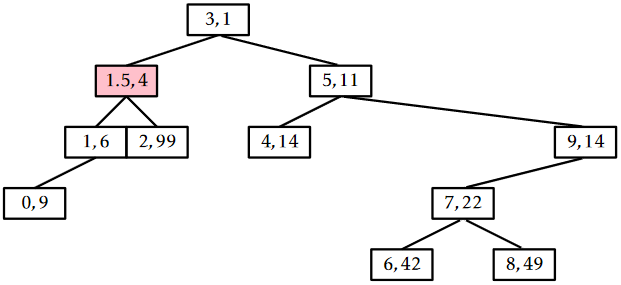
An example of the \(\mathtt{remove(x)}\) operation is shown in Figure \(\PageIndex{4}\).
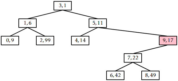
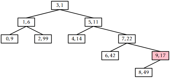
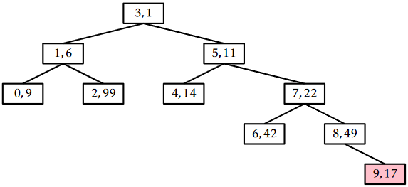
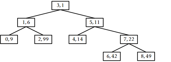
The trick to analyze the running time of the \(\mathtt{remove(x)}\) operation is to notice that this operation reverses the \(\mathtt{add(x)}\) operation. In particular, if we were to reinsert \(\mathtt{x}\), using the same priority \(\texttt{u.p}\), then the \(\mathtt{add(x)}\) operation would do exactly the same number of rotations and would restore the Treap to exactly the same state it was in before the \(\mathtt{remove(x)}\) operation took place. (Reading from bottom-to-top, Figure \(\PageIndex{4}\) illustrates the addition of the value 9 into a Treap.) This means that the expected running time of the \(\mathtt{remove(x)}\) on a Treap of size \(\mathtt{n}\) is proportional to the expected running time of the \(\mathtt{add(x)}\) operation on a Treap of size \(\mathtt{n}-1\). We conclude that the expected running time of \(\mathtt{remove(x)}\) is \(O(\log \mathtt{n})\).
\(\PageIndex{1}\) Summary
The following theorem summarizes the performance of the Treap data structure:
Theorem \(\PageIndex{1}\).
A Treap implements the SSet interface. A Treap supports the operations \(\mathtt{add(x)}\), \(\mathtt{remove(x)}\), and \(\mathtt{find(x)}\) in \(O(\log \mathtt{n})\) expected time per operation.
It is worth comparing the Treap data structure to the SkiplistSSet data structure. Both implement the SSet operations in \(O(\log \mathtt{n})\) expected time per operation. In both data structures, \(\mathtt{add(x)}\) and \(\mathtt{remove(x)}\) involve a search and then a constant number of pointer changes (see Exercise 7.3.5). Thus, for both these structures, the expected length of the search path is the critical value in assessing their performance. In a SkiplistSSet, the expected length of a search path is
\[ 2\log \mathtt{n} + O(1) \enspace , \nonumber\]
In a Treap, the expected length of a search path is
\[ 2\ln \mathtt{n} +O(1) \approx 1.386\log \mathtt{n} + O(1) \enspace . \nonumber\]
Thus, the search paths in a Treap are considerably shorter and this translates into noticeably faster operations on Treaps than Skiplists. Exercise 4.5.7 in Chapter 4 shows how the expected length of the search path in a Skiplist can be reduced to
\[ e\ln \mathtt{n} + O(1) \approx 1.884\log \mathtt{n} + O(1) \nonumber\]
by using biased coin tosses. Even with this optimization, the expected length of search paths in a SkiplistSSet is noticeably longer than in a Treap.
Footnotes
2The names Treap comes from the fact that this data structure is simultaneously a binary search tree (Section 6.2) and a heap (Chapter 10).
3The rank of an element \(\mathtt{x}\) in a set \(S\) of elements is the number of elements in \(S\) that are less than \(\mathtt{x}\).