11.2: Counting Sort and Radix Sort

In this section we study two sorting algorithms that are not comparison-based. Specialized for sorting small integers, these algorithms elude the lower-bounds of Theorem 11.1.5 by using (parts of) the elements in \(\mathtt{a}\) as indices into an array. Consider a statement of the form

\[ \mathtt{c[a[i]]} = 1 \enspace . \nonumber\]

This statement executes in constant time, but has \(\texttt{c.length}\) possible different outcomes, depending on the value of \(\mathtt{a[i]}\). This means that the execution of an algorithm that makes such a statement cannot be modelled as a binary tree. Ultimately, this is the reason that the algorithms in this section are able to sort faster than comparison-based algorithms.

\(\PageIndex{1}\) Counting Sort

Suppose we have an input array \(\mathtt{a}\) consisting of \(\mathtt{n}\) integers, each in the range \(0,\ldots,\mathtt{k}-1\). The counting-sort algorithm sorts \(\mathtt{a}\) using an auxiliary array \(\mathtt{c}\) of counters. It outputs a sorted version of \(\mathtt{a}\) as an auxiliary array \(\mathtt{b}\).

The idea behind counting-sort is simple: For each \(\mathtt{i}\in\{0,\ldots,\mathtt{k}-1\}\), count the number of occurrences of \(\mathtt{i}\) in \(\mathtt{a}\) and store this in \(\mathtt{c[i]}\). Now, after sorting, the output will look like \(\mathtt{c[0]}\) occurrences of 0, followed by \(\mathtt{c[1]}\) occurrences of 1, followed by \(\mathtt{c[2]}\) occurrences of 2,..., followed by \(\mathtt{c[k-1]}\) occurrences of \(\mathtt{k-1}\). The code that does this is very slick, and its execution is illustrated in Figure \(\PageIndex{1}\):

    int[] countingSort(int[] a, int k) {
        int c[] = new int[k];
        for (int i = 0; i < a.length; i++)
            c[a[i]]++;
        for (int i = 1; i < k; i++)
            c[i] += c[i-1];
        int b[] = new int[a.length];
        for (int i = a.length-1; i >= 0; i--)
            b[--c[a[i]]] = a[i];
        return b;
    }

Figure \(\PageIndex{1}\): The operation of counting sort on an array of length \(\mathtt{n}=20\) that stores integers \(0,\ldots,\mathtt{k}-1=9\).

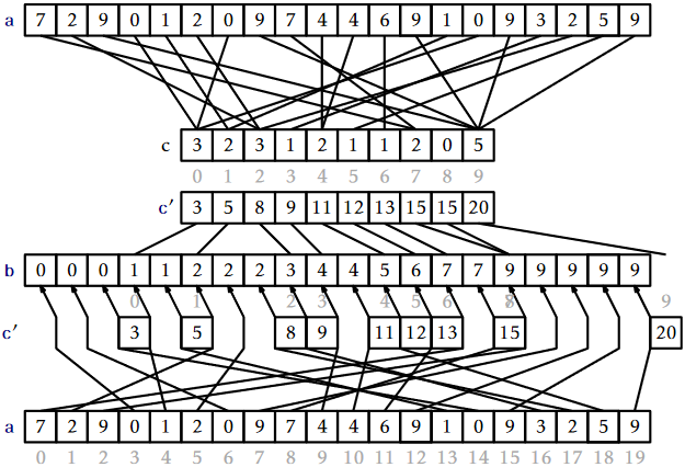
The first \(\mathtt{for}\) loop in this code sets each counter \(\mathtt{c[i]}\) so that it counts the number of occurrences of \(\mathtt{i}\) in \(\mathtt{a}\). By using the values of \(\mathtt{a}\) as indices, these counters can all be computed in \(O(\mathtt{n})\) time with a single for loop. At this point, we could use \(\mathtt{c}\) to fill in the output array \(\mathtt{b}\) directly. However, this would not work if the elements of \(\mathtt{a}\) have associated data. Therefore we spend a little extra effort to copy the elements of \(\mathtt{a}\) into \(\mathtt{b}\).

The next \(\mathtt{for}\) loop, which takes \(O(\mathtt{k})\) time, computes a running-sum of the counters so that \(\mathtt{c[i]}\) becomes the number of elements in \(\mathtt{a}\) that are less than or equal to \(\mathtt{i}\). In particular, for every \(\mathtt{i}\in\{0,\ldots,\mathtt{k}-1\}\), the output array, \(\mathtt{b}\), will have

\[ \mathtt{b[c[i-1]]}=\mathtt{b[c[i-1]+1]=}\cdots=\mathtt{b[c[i]-1]}=\mathtt{i} \enspace . \nonumber\]

Finally, the algorithm scans \(\mathtt{a}\) backwards to place its elements, in order, into an output array \(\mathtt{b}\). When scanning, the element \(\mathtt{a[i]=j}\) is placed at location \(\mathtt{b[c[j]-1]}\) and the value \(\mathtt{c[j]}\) is decremented.

Theorem \(\PageIndex{1}\).

The \(\mathtt{countingSort(a,k)}\) method can sort an array \(\mathtt{a}\) containing \(\mathtt{n}\) integers in the set \(\{0,\ldots,\mathtt{k}-1\}\) in \(O(\mathtt{n}+\mathtt{k})\) time.

The counting-sort algorithm has the nice property of being stable; it preserves the relative order of equal elements. If two elements \(\mathtt{a[i]}\) and \(\mathtt{a[j]}\) have the same value, and \(\mathtt{i}<\mathtt{j}\) then \(\mathtt{a[i]}\) will appear before \(\mathtt{a[j]}\) in \(\mathtt{b}\). This will be useful in the next section.

\(\PageIndex{2}\) Radix-Sort

Counting-sort is very efficient for sorting an array of integers when the length, \(\mathtt{n}\), of the array is not much smaller than the maximum value, \(\mathtt{k}-1\), that appears in the array. The radix-sort algorithm, which we now describe, uses several passes of counting-sort to allow for a much greater range of maximum values.

Radix-sort sorts \(\mathtt{w}\)-bit integers by using \(\mathtt{w}/\mathtt{d}\) passes of counting-sort to sort these integers \(\mathtt{d}\) bits at a time.² More precisely, radix sort first sorts the integers by their least significant \(\mathtt{d}\) bits, then their next significant \(\mathtt{d}\) bits, and so on until, in the last pass, the integers are sorted by their most significant \(\mathtt{d}\) bits.

    int[] radixSort(int[] a) {
        int[] b = null;
        for (int p = 0; p < w/d; p++) {
            int c[] = new int[1<<d];
            // the next three for loops implement counting-sort
            b = new int[a.length];
            for (int i = 0; i < a.length; i++)
                c[(a[i] >> d*p)&((1<<d)-1)]++;
            for (int i = 1; i < 1<<d; i++)
                c[i] += c[i-1];
            for (int i = a.length-1; i >= 0; i--)
                b[--c[(a[i] >> d*p)&((1<<d)-1)]] = a[i];
            a = b;
        }
        return b;
    }

(In this code, the expression \(\mathtt{(a[i]\text{>>}d*p)\text{&}((1\text{<<}d)-1)}\) extracts the integer whose binary representation is given by bits \((\mathtt{p}+1)\mathtt{d}-1,\ldots,\mathtt{p}\mathtt{d}\) of \(\mathtt{a[i]}\).) An example of the steps of this algorithm is shown in Figure \(\PageIndex{2}\).

Figure \(\PageIndex{2}\): Using radixsort to sort \(\mathtt{w}=8\)-bit integers by using 4 passes of counting sort on \(\mathtt{d}=2\)-bit integers.

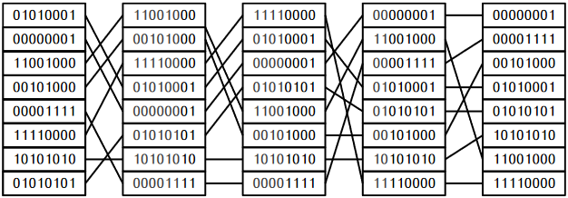
This remarkable algorithm sorts correctly because counting-sort is a stable sorting algorithm. If \(\mathtt{x} < \mathtt{y}\) are two elements of \(\mathtt{a}\), and the most significant bit at which \(\mathtt{x}\) differs from \(\mathtt{y}\) has index \(r\), then \(\mathtt{x}\) will be placed before \(\mathtt{y}\) during pass \(\lfloor r/\mathtt{d}\rfloor\) and subsequent passes will not change the relative order of \(\mathtt{x}\) and \(\mathtt{y}\).

Radix-sort performs \(\mathtt{w/d}\) passes of counting-sort. Each pass requires \(O(\mathtt{n}+2^{\mathtt{d}})\) time. Therefore, the performance of radix-sort is given by the following theorem.

Theorem \(\PageIndex{2}\).

For any integer \(\mathtt{d}>0\), the \(\mathtt{radixSort(a,k)}\) method can sort an array \(\mathtt{a}\) containing \(\mathtt{n}\) \(\mathtt{w}\)-bit integers in \(O((\mathtt{w}/\mathtt{d})(\mathtt{n}+2^{\mathtt{d}}))\) time.

If we think, instead, of the elements of the array being in the range \(\{0,\ldots,\mathtt{n}^c-1\}\), and take \(\mathtt{d}=\lceil\log\mathtt{n}\rceil\) we obtain the following version of Theorem \(\PageIndex{2}\).

Corollary \(\PageIndex{1}\).

The \(\mathtt{radixSort(a,k)}\) method can sort an array \(\mathtt{a}\) containing \(\mathtt{n}\) integer values in the range \(\{0,\ldots,\mathtt{n}^c-1\}\) in \(O(c\mathtt{n})\) time.

---

Footnotes

²We assume that \(\mathtt{d}\) divides \(\mathtt{w}\), otherwise we can always increase \(\mathtt{w}\) to \(\mathtt{d}\lceil\mathtt{w}/\mathtt{d}\rceil\).