9.4: Discussion and Exercises
- Page ID
- 8475
Red-black trees were first introduced by Guibas and Sedgewick [38]. Despite their high implementation complexity they are found in some of the most commonly used libraries and applications. Most algorithms and data structures textbooks discuss some variant of red-black trees.
Andersson [6] describes a left-leaning version of balanced trees that is similar to red-black trees but has the additional constraint that any node has at most one red child. This implies that these trees simulate 2-3 trees rather than 2-4 trees. They are significantly simpler, though, than the RedBlackTree structure presented in this chapter.
Sedgewick [66] describes two versions of left-leaning red-black trees. These use recursion along with a simulation of top-down splitting and merging in 2-4 trees. The combination of these two techniques makes for particularly short and elegant code.
A related, and older, data structure is the AVL tree [3]. AVL trees are height-balanced: At each node \(u\), the height of the subtree rooted at \(\texttt{u.left}\) and the subtree rooted at \(\texttt{u.right}\) differ by at most one. It follows immediately that, if \(F(h)\) is the minimum number of leaves in a tree of height \(h\), then \(F(h)\) obeys the Fibonacci recurrence
\[ F(h) = F(h-1) + F(h-2) \nonumber\]
with base cases \(F(0)=1\) and \(F(1)=1\). This means \(F(h)\) is approximately \(\varphi^h/\sqrt{5}\), where \(\varphi=(1+\sqrt{5})/2\approx1.61803399\) is the golden ratio. (More precisely, \(\vert\varphi^h/\sqrt{5} - F(h)\vert\le 1/2\).) Arguing as in the proof of Lemma 9.1.1, this implies
\[ h \le \log_\varphi \mathtt{n} \approx 1.440420088\log \mathtt{n} \enspace , \nonumber\]
so AVL trees have smaller height than red-black trees. The height balancing can be maintained during \(\mathtt{add(x)}\) and \(\mathtt{remove(x)}\) operations by walking back up the path to the root and performing a rebalancing operation at each node \(\mathtt{u}\) where the height of \(\mathtt{u}\)'s left and right subtrees differ by two. See Figure \(\PageIndex{1}\).

Andersson's variant of red-black trees, Sedgewick's variant of red-black trees, and AVL trees are all simpler to implement than the RedBlackTree structure defined here. Unfortunately, none of them can guarantee that the amortized time spent rebalancing is \(O(1)\) per update. In particular, there is no analogue of Theorem 9.3.2 for those structures.

Exercise \(\PageIndex{1}\)
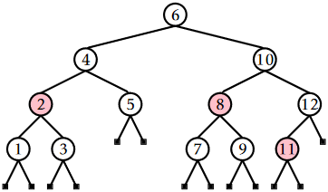
Illustrate the 2-4 tree that corresponds to the RedBlackTree in Figure \(\PageIndex{2}\).
Exercise \(\PageIndex{2}\)
Illustrate the addition of 13, then 3.5, then 3.3 on the RedBlackTree in Figure \(\PageIndex{2}\).
Exercise \(\PageIndex{3}\)
Illustrate the removal of 11, then 9, then 5 on the RedBlackTree in Figure \(\PageIndex{2}\).
Exercise \(\PageIndex{4}\)
Show that, for arbitrarily large values of \(\mathtt{n}\), there are red-black trees with \(\mathtt{n}\) nodes that have height \(2\log \mathtt{n}-O(1)\).
Exercise \(\PageIndex{5}\)
Consider the operations \(\mathtt{pushBlack(u)}\) and \(\mathtt{pullBlack(u)}\). What do these operations do to the underlying 2-4 tree that is being simulated by the red-black tree?
Exercise \(\PageIndex{6}\)
Show that, for arbitrarily large values of \(\mathtt{n}\), there exist sequences of \(\mathtt{add(x)}\) and \(\mathtt{remove(x)}\) operations that lead to red-black trees with \(\mathtt{n}\) nodes that have height \(2\log \mathtt{n}-O(1)\).
Exercise \(\PageIndex{7}\)
Why does the method \(\mathtt{remove(x)}\) in the RedBlackTree implementation perform the assignment \(\mathtt{u.parent=w.parent}\)? Shouldn't this already be done by the call to \(\mathtt{splice(w)}\)?
Exercise \(\PageIndex{8}\)
Suppose a 2-4 tree, \(T\), has \(\mathtt{n}_\ell\) leaves and \(\mathtt{n}_i\) internal nodes.
- What is the minimum value of \(\mathtt{n}_i\), as a function of \(\mathtt{n}_\ell\)?
- What is the maximum value of \(\mathtt{n}_i\), as a function of \(\mathtt{n}_\ell\)?
- If \(T'\) is a red-black tree that represents \(T\), then how many red nodes does \(T'\) have?
Exercise \(\PageIndex{9}\)
Suppose you are given a binary search tree with \(\mathtt{n}\) nodes and a height of at most \(2\log \mathtt{n}-2\). Is it always possible to colour the nodes red and black so that the tree satisfies the black-height and no-red-edge properties? If so, can it also be made to satisfy the left-leaning property?
Suppose you have two red-black trees \(T_1\) and \(T_2\) that have the same black height, \(h\), and such that the largest key in \(T_1\) is smaller than the smallest key in \(T_2\). Show how to merge \(T_1\) and \(T_2\) into a single red-black tree in \(O(h)\) time.
Exercise \(\PageIndex{11}\)
Extend your solution to Exercise \(\PageIndex{10}\) to the case where the two trees \(T_1\) and \(T_2\) have different black heights, \(h_1\neq h_2\). The running-time should be \(O(\max\{h_1,h_2\})\).
Exercise \(\PageIndex{12}\)
Prove that, during an \(\mathtt{add(x)}\) operation, an AVL tree must perform at most one rebalancing operation (that involves at most two rotations; see Figure \(\PageIndex{1}\)). Give an example of an AVL tree and a \(\mathtt{remove(x)}\) operation on that tree that requires on the order of \(\log\mathtt{n}\) rebalancing operations.
Exercise \(\PageIndex{13}\)
Implement an AVLTree class that implements AVL trees as described above. Compare its performance to that of the RedBlackTree implementation. Which implementation has a faster \(\mathtt{find(x)}\) operation?
Exercise \(\PageIndex{14}\)
Design and implement a series of experiments that compare the relative performance of \(\mathtt{find(x)}\), \(\mathtt{add(x)}\), and \(\mathtt{remove(x)}\) for the SSet implemeentations SkiplistSSet, ScapegoatTree, Treap, and RedBlackTree. Be sure to include multiple test scenarios, including cases where the data is random, already sorted, is removed in random order, is removed in sorted order, and so on.


