12.4: Discussion and Exercises

Last updated
Save as PDF

Page ID: 8488

$ \newcommand{\vecs}[1]{\overset { \scriptstyle \rightharpoonup} {\mathbf{#1}} } $ $ \newcommand{\vecd}[1]{\overset{-\!-\!\rightharpoonup}{\vphantom{a}\smash {#1}}} $$\newcommand{\id}{\mathrm{id}}$ $ \newcommand{\Span}{\mathrm{span}}$ $ \newcommand{\kernel}{\mathrm{null}\,}$ $ \newcommand{\range}{\mathrm{range}\,}$ $ \newcommand{\RealPart}{\mathrm{Re}}$ $ \newcommand{\ImaginaryPart}{\mathrm{Im}}$ $ \newcommand{\Argument}{\mathrm{Arg}}$ $ \newcommand{\norm}[1]{\| #1 \|}$ $ \newcommand{\inner}[2]{\langle #1, #2 \rangle}$ $ \newcommand{\Span}{\mathrm{span}}$ $\newcommand{\id}{\mathrm{id}}$ $ \newcommand{\Span}{\mathrm{span}}$ $ \newcommand{\kernel}{\mathrm{null}\,}$ $ \newcommand{\range}{\mathrm{range}\,}$ $ \newcommand{\RealPart}{\mathrm{Re}}$ $ \newcommand{\ImaginaryPart}{\mathrm{Im}}$ $ \newcommand{\Argument}{\mathrm{Arg}}$ $ \newcommand{\norm}[1]{\| #1 \|}$ $ \newcommand{\inner}[2]{\langle #1, #2 \rangle}$ $ \newcommand{\Span}{\mathrm{span}}$$\newcommand{\AA}{\unicode[.8,0]{x212B}}$

The running times of the depth-first-search and breadth-first-search algorithms are somewhat overstated by the Theorems 12.3.1 and 12.3.2. Define $\mathtt{n}_{\mathtt{r}}$ as the number of vertices, $\mathtt{i}$, of $G$, for which there exists a path from $\mathtt{r}$ to $\mathtt{i}$. Define $\mathtt{m}_\mathtt{r}$ as the number of edges that have these vertices as their sources. Then the following theorem is a more precise statement of the running times of the breadth-first-search and depth-first-search algorithms. (This more refined statement of the running time is useful in some of the applications of these algorithms outlined in the exercises.)

Theorem $\PageIndex{1}$

When given as input a Graph, $\mathtt{g}$, that is implemented using the AdjacencyLists data structure, the $\mathtt{bfs(g,r)}$, $\mathtt{dfs(g,r)}$ and $\mathtt{dfs2(g,r)}$ algorithms each run in $O(\mathtt{n}_{\mathtt{r}}+\mathtt{m}_{\mathtt{r}})$ time.

Breadth-first search seems to have been discovered independently by Moore [52] and Lee [49] in the contexts of maze exploration and circuit routing, respectively.

Adjacency-list representations of graphs were presented by Hopcroft and Tarjan [40] as an alternative to the (then more common) adjacency-matrix representation. This representation, as well as depth-first-search, played a major part in the celebrated Hopcroft-Tarjan planarity testing algorithm that can determine, in $O(\mathtt{n})$ time, if a graph can be drawn, in the plane, and in such a way that no pair of edges cross each other [41].

In the following exercises, an undirected graph is one in which, for every $\mathtt{i}$ and $\mathtt{j}$, the edge $(\mathtt{i},\mathtt{j})$ is present if and only if the edge $(\mathtt{j},\mathtt{i})$ is present.

Exercise $\PageIndex{1}$

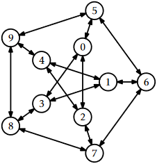
Draw an adjacency list representation and an adjacency matrix representation of the graph in Figure $\PageIndex{1}$.

Figure $\PageIndex{1}$: An example graph.

Exercise $\PageIndex{2}$

The incidence matrix representation of a graph, $G$, is an $\mathtt{n}\times\mathtt{m}$ matrix, $A$, where

\[\displaystyle A_{i,j} =
\begin{cases}
-1 & \text{if vertex $i$ the source of edge $j$} \\
+1 & \text{if vertex $i$ the target of edge $j$} \\
0 & \text{otherwise.}
\end{cases}\nonumber\]

Draw the incident matrix representation of the graph in Figure $\PageIndex{1}$.
Design, analyze and implement an incidence matrix representation of a graph. Be sure to analyze the space, the cost of $\mathtt{addEdge(i,j)}$, $\mathtt{removeEdge(i,j)}$, $\mathtt{hasEdge(i,j)}$, $\mathtt{inEdges(i)}$, and $\mathtt{outEdges(i)}$.

Exercise $\PageIndex{3}$

Illustrate an execution of the $\mathtt{bfs(G,0)}$ and $\mathtt{dfs(G,0)}$ on the graph, $\mathtt{G}$, in Figure $\PageIndex{1}$.

Exercise $\PageIndex{4}$

Let $G$ be an undirected graph. We say $G$ is connected if, for every pair of vertices $\mathtt{i}$ and $\mathtt{j}$ in $G$, there is a path from $\mathtt{i}$ to $\mathtt{j}$ (since $G$ is undirected, there is also a path from $\mathtt{j}$ to $\mathtt{i}$). Show how to test if $G$ is connected in $O(\mathtt{n}+\mathtt{m})$ time.

Exercise $\PageIndex{5}$

Let $G$ be an undirected graph. A connected-component labelling of $G$ partitions the vertices of $G$ into maximal sets, each of which forms a connected subgraph. Show how to compute a connected component labelling of $G$ in $O(\mathtt{n}+\mathtt{m})$ time.

Exercise $\PageIndex{6}$

Let $G$ be an undirected graph. A spanning forest of $G$ is a collection of trees, one per component, whose edges are edges of $G$ and whose vertices contain all vertices of $G$. Show how to compute a spanning forest of of $G$ in $O(\mathtt{n}+\mathtt{m})$ time.

Exercise $\PageIndex{7}$

We say that a graph $G$ is strongly-connected if, for every pair of vertices $\mathtt{i}$ and $\mathtt{j}$ in $G$, there is a path from $\mathtt{i}$ to $\mathtt{j}$. Show how to test if $G$ is strongly-connected in $O(\mathtt{n}+\mathtt{m})$ time.

Exercise $\PageIndex{8}$

Given a graph $G=(V,E)$ and some special vertex $\mathtt{r}\in V$, show how to compute the length of the shortest path from $\mathtt{r}$ to $\mathtt{i}$ for every vertex $\mathtt{i}\in V$.

Exercise $\PageIndex{9}$

Give a (simple) example where the $\mathtt{dfs(g,r)}$ code visits the nodes of a graph in an order that is different from that of the $\mathtt{dfs2(g,r)}$ code. Write a version of $\mathtt{dfs2(g,r)}$ that always visits nodes in exactly the same order as $\mathtt{dfs(g,r)}$. (Hint: Just start tracing the execution of each algorithm on some graph where $\mathtt{r}$ is the source of more than 1 edge.)

Exercise $\PageIndex{10}$

A universal sink in a graph $G$ is a vertex that is the target of $\mathtt{n}-1$ edges and the source of no edges.¹ Design and implement an algorithm that tests if a graph $G$, represented as an AdjacencyMatrix, has a universal sink. Your algorithm should run in $O(\mathtt{n})$ time.

Footnotes

¹A universal sink, $\mathtt{v}$, is also sometimes called a celebrity: Everyone in the room recognizes $\mathtt{v}$, but $\mathtt{v}$ doesn't recognize anyone else in the room.