13.3: YFastTrie - A Doubly-Logarithmic Time SSet
- Page ID
- 8492
The XFastTrie is a vast--even exponential--improvement over the BinaryTrie in terms of query time, but the \(\mathtt{add(x)}\) and \(\mathtt{remove(x)}\) operations are still not terribly fast. Furthermore, the space usage, \(O(\mathtt{n}\cdot\mathtt{w})\), is higher than the other SSet implementations described in this book, which all use \(O(\mathtt{n})\) space. These two problems are related; if \(\mathtt{n}\) \(\mathtt{add(x)}\) operations build a structure of size \(\mathtt{n}\cdot\mathtt{w}\), then the \(\mathtt{add(x)}\) operation requires at least on the order of \(\mathtt{w}\) time (and space) per operation.
The YFastTrie, discussed next, simultaneously improves the space and speed of XFastTries. A YFastTrie uses an XFastTrie, \(\mathtt{xft}\), but only stores \(O(\mathtt{n}/\mathtt{w})\) values in \(\mathtt{xft}\). In this way, the total space used by \(\mathtt{xft}\) is only \(O(\mathtt{n})\). Furthermore, only one out of every \(\mathtt{w}\) \(\mathtt{add(x)}\) or \(\mathtt{remove(x)}\) operations in the YFastTrie results in an \(\mathtt{add(x)}\) or \(\mathtt{remove(x)}\) operation in \(\mathtt{xft}\). By doing this, the average cost incurred by calls to \(\mathtt{xft}\)'s \(\mathtt{add(x)}\) and \(\mathtt{remove(x)}\) operations is only constant.
The obvious question becomes: If \(\mathtt{xft}\) only stores \(\mathtt{n}\)/\(\mathtt{w}\) elements, where do the remaining \(\mathtt{n}(1-1/\mathtt{w})\) elements go? These elements move into secondary structures, in this case an extended version of treaps (Section 7.2). There are roughly \(\mathtt{n}\)/\(\mathtt{w}\) of these secondary structures so, on average, each of them stores \(O(\mathtt{w})\) items. Treaps support logarithmic time SSet operations, so the operations on these treaps will run in \(O(\log \mathtt{w})\) time, as required.
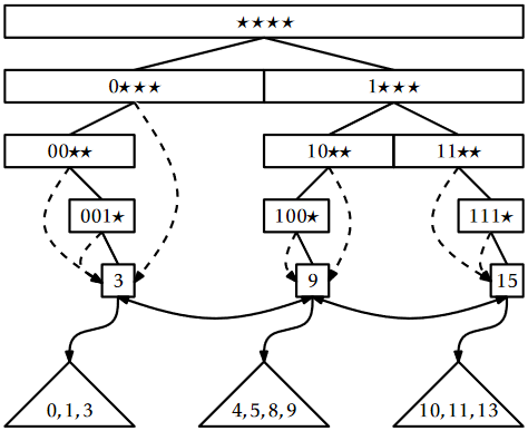
More concretely, a YFastTrie contains an XFastTrie, \(\mathtt{xft}\), that contains a random sample of the data, where each element appears in the sample independently with probability \(1/\mathtt{w}\). For convenience, the value \(2^{\mathtt{w}}-1\), is always contained in \(\mathtt{xft}\). Let \(\mathtt{x}_0<\mathtt{x}_1<\cdots<\mathtt{x}_{k-1}\) denote the elements stored in \(\mathtt{xft}\). Associated with each element, \(\mathtt{x}_i\), is a treap, \(\mathtt{t}_i\), that stores all values in the range \(\mathtt{x}_{i-1}+1,\ldots,\mathtt{x}_i\). This is illustrated in Figure \(\PageIndex{1}\).

The \(\mathtt{find(x)}\) operation in a YFastTrie is fairly easy. We search for \(\mathtt{x}\) in \(\mathtt{xft}\) and find some value \(\mathtt{x}_i\) associated with the treap \(\mathtt{t}_i\). We then use the treap \(\mathtt{find(x)}\) method on \(\mathtt{t}_i\) to answer the query. The entire method is a one-liner:
    T find(T x) {
        return xft.find(new Pair<T>(it.intValue(x))).t.find(x);
    }
The first \(\mathtt{find(x)}\) operation (on \(\mathtt{xft}\)) takes \(O(\log\mathtt{w})\) time. The second \(\mathtt{find(x)}\) operation (on a treap) takes \(O(\log r)\) time, where \(r\) is the size of the treap. Later in this section, we will show that the expected size of the treap is \(O(\mathtt{w})\) so that this operation takes \(O(\log \mathtt{w})\) time.1
Adding an element to a YFastTrie is also fairly simple--most of the time. The \(\mathtt{add(x)}\) method calls \(\texttt{xft.find(x)}\) to locate the treap, \(\mathtt{t}\), into which \(\mathtt{x}\) should be inserted. It then calls \(\texttt{t.add(x)}\) to add \(\mathtt{x}\) to \(\mathtt{t}\). At this point, it tosses a biased coin that comes up as heads with probability \(1/\mathtt{w}\) and as tails with probability \(1-1/\mathtt{w}\). If this coin comes up heads, then \(\mathtt{x}\) will be added to \(\mathtt{xft}\).
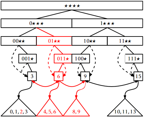
This is where things get a little more complicated. When \(\mathtt{x}\) is added to \(\mathtt{xft}\), the treap \(\mathtt{t}\) needs to be split into two treaps, \(\mathtt{t1}\) and \(\mathtt{t'}\). The treap \(\mathtt{t1}\) contains all the values less than or equal to \(\mathtt{x}\); \(\mathtt{t'}\) is the original treap, \(\mathtt{t}\), with the elements of \(\mathtt{t1}\) removed. Once this is done, we add the pair \(\mathtt{(x,t1)}\) to \(\mathtt{xft}\). Figure \(\PageIndex{2}\) shows an example.
    boolean add(T x) {
        int ix = it.intValue(x);
        STreap<T> t = xft.find(new Pair<T>(ix)).t;
        if (t.add(x)) {
            n++;
            if (rand.nextInt(w) == 0) {
                STreap<T> t1 = t.split(x);
                xft.add(new Pair<T>(ix, t1));
            }
            return true;
        }
        return false;
    }

Adding \(\mathtt{x}\) to \(\mathtt{t}\) takes \(O(\log \mathtt{w})\) time. Exercise 7.3.12 shows that splitting \(\mathtt{t}\) into \(\mathtt{t1}\) and \(\mathtt{t'}\) can also be done in \(O(\log \mathtt{w})\) expected time. Adding the pair (\(\mathtt{x}\), \(\mathtt{t1}\)) to \(\mathtt{xft}\) takes \(O(\mathtt{w})\) time, but only happens with probability \(1/\mathtt{w}\). Therefore, the expected running time of the \(\mathtt{add(x)}\) operation is
\[ O(\log\mathtt{w}) + \frac{1}{\mathtt{w}}O(\mathtt{w}) = O(\log \mathtt{w}) \enspace . \nonumber\]
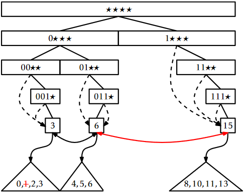
The \(\mathtt{remove(x)}\) method undoes the work performed by \(\mathtt{add(x)}\). We use \(\mathtt{xft}\) to find the leaf, \(\mathtt{u}\), in \(\mathtt{xft}\) that contains the answer to \(\texttt{xft.find(x)}\). From \(\mathtt{u}\), we get the treap, \(\mathtt{t}\), containing \(\mathtt{x}\) and remove \(\mathtt{x}\) from \(\mathtt{t}\). If \(\mathtt{x}\) was also stored in \(\mathtt{xft}\) (and \(\mathtt{x}\) is not equal to \(2^{\mathtt{w}}-1\)) then we remove \(\mathtt{x}\) from \(\mathtt{xft}\) and add the elements from \(\mathtt{x}\)'s treap to the treap, \(\mathtt{t2}\), that is stored by \(\mathtt{u}\)'s successor in the linked list. This is illustrated in Figure \(\PageIndex{3}\).
    boolean remove(T x) {
        int ix = it.intValue(x);
        Node<T> u = xft.findNode(ix);
        boolean ret = u.x.t.remove(x);
        if (ret) n--;
        if (u.x.x == ix && ix != 0xffffffff) {
            STreap<T> t2 = u.child[1].x.t;
            t2.absorb(u.x.t);
            xft.remove(u.x);
        }
        return ret;
    }

Finding the node \(\mathtt{u}\) in \(\mathtt{xft}\) takes \(O(\log\mathtt{w})\) expected time. Removing \(\mathtt{x}\) from \(\mathtt{t}\) takes \(O(\log\mathtt{w})\) expected time. Again, Exercise 7.3.12 shows that merging all the elements of \(\mathtt{t}\) into \(\mathtt{t2}\) can be done in \(O(\log\mathtt{w})\) time. If necessary, removing \(\mathtt{x}\) from \(\mathtt{xft}\) takes \(O(\mathtt{w})\) time, but \(\mathtt{x}\) is only contained in \(\mathtt{xft}\) with probability \(1/\mathtt{w}\). Therefore, the expected time to remove an element from a YFastTrie is \(O(\log \mathtt{w})\).
Earlier in the discussion, we delayed arguing about the sizes of treaps in this structure until later. Before finishing this chapter, we prove the result we need.
Let \(\mathtt{x}\) be an integer stored in a YFastTrie and let \(\mathtt{n}_\mathtt{x}\) denote the number of elements in the treap, \(\mathtt{t}\), that contains \(\mathtt{x}\). Then \(\mathrm{E}[\mathtt{n}_\mathtt{x}] \le 2\mathtt{w}-1\).
Proof. Refer to Figure \(\PageIndex{4}\). Let \(\mathtt{x}_1<\mathtt{x}_2<\cdots<\mathtt{x}_{i}=\mathtt{x}<\mathtt{x}_{i+1}<\cdots<\mathtt{x}_\mathtt{n}\) denote the elements stored in the YFastTrie. The treap \(\mathtt{t}\) contains some elements greater than or equal to \(\mathtt{x}\). These are \(\mathtt{x}_i,\mathtt{x}_{i+1},\ldots,\mathtt{x}_{i+j-1}\), where \(\mathtt{x}_{i+j-1}\) is the only one of these elements in which the biased coin toss performed in the \(\mathtt{add(x)}\) method turned up as heads. In other words, \(\mathrm{E}[j]\) is equal to the expected number of biased coin tosses required to obtain the first heads.2 Each coin toss is independent and turns up as heads with probability \(1/\mathtt{w}\), so \(\mathrm{E}[j]\le\mathtt{w}\). (See Lemma 4.4.1 for an analysis of this for the case \(\mathtt{w}=2\).)
Similarly, the elements of \(\mathtt{t}\) smaller than \(\mathtt{x}\) are \(\mathtt{x}_{i-1},\ldots,\mathtt{x}_{i-k}\) where all these \(k\) coin tosses turn up as tails and the coin toss for \(\mathtt{x}_{i-k-1}\) turns up as heads. Therefore, \(\mathrm{E}[k]\le\mathtt{w}-1\), since this is the same coin tossing experiment considered in the preceding paragraph, but one in which the last toss is not counted. In summary, \(\mathtt{n}_\mathtt{x}=j+k\), so
\[ \mathrm{E}[\mathtt{n}_\mathtt{x}] = \mathrm{E}[j+k]= \mathrm{E}[j] + \mathrm{E}[k] \le 2\mathtt{w}-1 \enspace . \nonumber\]
![]()

Lemma \(\PageIndex{1}\) was the last piece in the proof of the following theorem, which summarizes the performance of the YFastTrie:
Theorem \(\PageIndex{1}\).
A YFastTrie implements the SSet interface for \(\mathtt{w}\)-bit integers. A YFastTrie supports the operations \(\mathtt{add(x)}\), \(\mathtt{remove(x)}\), and \(\mathtt{find(x)}\) in \(O(\log \mathtt{w})\) expected time per operation. The space used by a YFastTrie that stores \(\mathtt{n}\) values is \(O(\mathtt{n}+\mathtt{w})\).
The \(\mathtt{w}\) term in the space requirement comes from the fact that \(\mathtt{xft}\) always stores the value \(2^\mathtt{w}-1\). The implementation could be modified (at the expense of adding some extra cases to the code) so that it is unnecessary to store this value. In this case, the space requirement in the theorem becomes \(O(\mathtt{n})\).
Footnotes
1This is an application of Jensen's Inequality: If \(\mathrm{E}[r]=\mathtt{w}\), then \(\mathrm{E}[\log r]\le \log w\).
2This analysis ignores the fact that \(j\) never exceeds \(\mathtt{n}-i+1\). However, this only decreases \(\mathrm{E}[j]\), so the upper bound still holds.


