4.1: Global Internet

Last updated
Save as PDF

Page ID: 13962

$ \newcommand{\vecs}[1]{\overset { \scriptstyle \rightharpoonup} {\mathbf{#1}} } $ $ \newcommand{\vecd}[1]{\overset{-\!-\!\rightharpoonup}{\vphantom{a}\smash {#1}}} $$\newcommand{\id}{\mathrm{id}}$ $ \newcommand{\Span}{\mathrm{span}}$ $ \newcommand{\kernel}{\mathrm{null}\,}$ $ \newcommand{\range}{\mathrm{range}\,}$ $ \newcommand{\RealPart}{\mathrm{Re}}$ $ \newcommand{\ImaginaryPart}{\mathrm{Im}}$ $ \newcommand{\Argument}{\mathrm{Arg}}$ $ \newcommand{\norm}[1]{\| #1 \|}$ $ \newcommand{\inner}[2]{\langle #1, #2 \rangle}$ $ \newcommand{\Span}{\mathrm{span}}$ $\newcommand{\id}{\mathrm{id}}$ $ \newcommand{\Span}{\mathrm{span}}$ $ \newcommand{\kernel}{\mathrm{null}\,}$ $ \newcommand{\range}{\mathrm{range}\,}$ $ \newcommand{\RealPart}{\mathrm{Re}}$ $ \newcommand{\ImaginaryPart}{\mathrm{Im}}$ $ \newcommand{\Argument}{\mathrm{Arg}}$ $ \newcommand{\norm}[1]{\| #1 \|}$ $ \newcommand{\inner}[2]{\langle #1, #2 \rangle}$ $ \newcommand{\Span}{\mathrm{span}}$$\newcommand{\AA}{\unicode[.8,0]{x212B}}$

4.1 Global Internet

At this point, we have seen how to connect a heterogeneous collection of networks to create an internetwork and how to use the simple hierarchy of the IP address to make routing in an internet somewhat scalable. We say "somewhat" scalable because, even though each router does not need to know about all the hosts connected to the internet, it does, in the model described so far, need to know about all the networks connected to the internet. Today's Internet has hundreds of thousands of networks connected to it (or more, depending on how you count). Routing protocols such as those we have just discussed do not scale to those kinds of numbers. This section looks at a variety of techniques that greatly improve scalability and that have enabled the Internet to grow as far as it has.

The tree structure of the Internet in 1990.

Before getting to these techniques, we need to have a general picture in our heads of what the global Internet looks like. It is not just a random interconnection of Ethernets, but instead it takes on a shape that reflects the fact that it interconnects many different organizations. Figure 1 gives a simple depiction of the state of the Internet in 1990. Since that time, the Internet's topology has grown much more complex than this figure suggests—we present a slightly more accurate picture of the current Internet in a later section—but this picture will do for now.

One of the salient features of this topology is that it consists of end-user sites (e.g., Stanford University) that connect to service provider networks (e.g., BARRNET was a provider network that served sites in the San Francisco Bay Area). In 1990, many providers served a limited geographic region and were thus known as regional networks. The regional networks were, in turn, connected by a nationwide backbone. In 1990, this backbone was funded by the National Science Foundation (NSF) and was therefore called the NSFNET backbone.

NSFNET gave way to Internet2, which still runs a backbone on behalf of Research and Education institutions in the US (there are similar R&E networks in other countries), but of course most people get their Internet connectivity from commercial providers. Although the detail is not shown in the figure, today the largest provider networks (they are called tier-1) are typically built from dozens of high-end routers located in major meteropolitan areas (colloquially referred to as "NFL cities") connected by point-to-point links (often with 100 Gbps capacity). Similarly, each end-user site is typically not a single network but instead consists of multiple physical networks connected by switches and routers.

Notice in that each provider and end-user is likely to be an administratively independent entity. This has some significant consequences on routing. For example, it is quite likely that different providers will have different ideas about the best routing protocol to use within their networks and on how metrics should be assigned to links in their network. Because of this independence, each provider's network is usually a single autonomous system (AS). We will define this term more precisely in a later section, but for now it is adequate to think of an AS as a network that is administered independently of other ASs.

The fact that the Internet has a discernible structure can be used to our advantage as we tackle the problem of scalability. In fact, we need to deal with two related scaling issues. The first is the scalability of routing. We need to find ways to minimize the number of network numbers that get carried around in routing protocols and stored in the routing tables of routers. The second is address utilization—that is, making sure that the IP address space does not get consumed too quickly.

Throughout this book, we see the principle of hierarchy used again and again to improve scalability. We saw in the previous chapter how the hierarchical structure of IP addresses, especially with the flexibility provided by Classless Interdomain Routing (CIDR) and subnetting, can improve the scalability of routing. In the next two sections, we'll see further uses of hierarchy (and its partner, aggregation) to provide greater scalability, first in a single domain and then between domains. Our final subsection looks at IP version 6, the invention of which was largely the result of scalability concerns.

Routing Areas

As a first example of using hierarchy to scale up the routing system, we'll examine how link-state routing protocols (such as OSPF and IS-IS) can be used to partition a routing domain into subdomains called areas. (The terminology varies somewhat among protocols—we use the OSPF terminology here.) By adding this extra level of hierarchy, we enable single domains to grow larger without overburdening the routing protocols or resorting to the more complex interdomain routing protocols described later.

An area is a set of routers that are administratively configured to exchange link-state information with each other. There is one special area—the backbone area, also known as area 0. An example of a routing domain divided into areas is shown in Figure 2 . Routers R1, R2, and R3 are members of the backbone area. They are also members of at least one nonbackbone area; R1 is actually a member of both area 1 and area 2. A router that is a member of both the backbone area and a nonbackbone area is an area border router (ABR). Note that these are distinct from the routers that are at the edge of an AS, which are referred to as AS border routers for clarity.

Routing within a single area is exactly as described in the previous chapter. All the routers in the area send link-state advertisements to each other and thus develop a complete, consistent map of the area. However, the link-state advertisements of routers that are not area border routers do not leave the area in which they originated. This has the effect of making the flooding and route calculation processes considerably more scalable. For example, router R4 in area 3 will never see a link-state advertisement from router R8 in area 1. As a consequence, it will know nothing about the detailed topology of areas other than its own.

How, then, does a router in one area determine the right next hop for a packet destined to a network in another area? The answer to this becomes clear if we imagine the path of a packet that has to travel from one nonbackbone area to another as being split into three parts. First, it travels from its source network to the backbone area, then it crosses the backbone, then it travels from the backbone to the destination network. To make this work, the area border routers summarize routing information that they have learned from one area and make it available in their advertisements to other areas. For example, R1 receives link-state advertisements from all the routers in area 1 and can thus determine the cost of reaching any network in area 1. When R1 sends link-state advertisements into area 0, it advertises the costs of reaching the networks in area 1 much as if all those networks were directly connected to R1. This enables all the area 0 routers to learn the cost to reach all networks in area 1. The area border routers then summarize this information and advertise it into the nonbackbone areas. Thus, all routers learn how to reach all networks in the domain.

Note that, in the case of area 2, there are two ABRs and that routers in area 2 will thus have to make a choice as to which one they use to reach the backbone. This is easy enough, since both R1 and R2 will be advertising costs to various networks, so it will become clear which is the better choice as the routers in area 2 run their shortest-path algorithm. For example, it is pretty clear that R1 is going to be a better choice than R2 for destinations in area 1.

When dividing a domain into areas, the network administrator makes a tradeoff between scalability and optimality of routing. The use of areas forces all packets traveling from one area to another to go via the backbone area, even if a shorter path might have been available. For example, even if R4 and R5 were directly connected, packets would not flow between them because they are in different nonbackbone areas. It turns out that the need for scalability is often more important than the need to use the absolute shortest path.

Key Takeaway

This illustrates an important principle in network design. There is frequently a trade-off between scalability and some sort of optimality. When hierarchy is introduced, information is hidden from some nodes in the network, hindering their ability to make perfect decisions. However, information hiding is essential to scalability, since it saves all nodes from having global knowledge. It is invariably true in large networks that scalability is a more pressing design goal than selecting the optimal route.

Finally, we note that there is a trick by which network administrators can more flexibly decide which routers go in area 0. This trick uses the idea of a virtual link between routers. Such a virtual link is obtained by configuring a router that is not directly connected to area 0 to exchange backbone routing information with a router that is. For example, a virtual link could be configured from R8 to R1, thus making R8 part of the backbone. R8 would now participate in link-state advertisement flooding with the other routers in area 0. The cost of the virtual link from R8 to R1 is determined by the exchange of routing information that takes place in area 1. This technique can help to improve the optimality of routing.

Interdomain Routing (BGP)

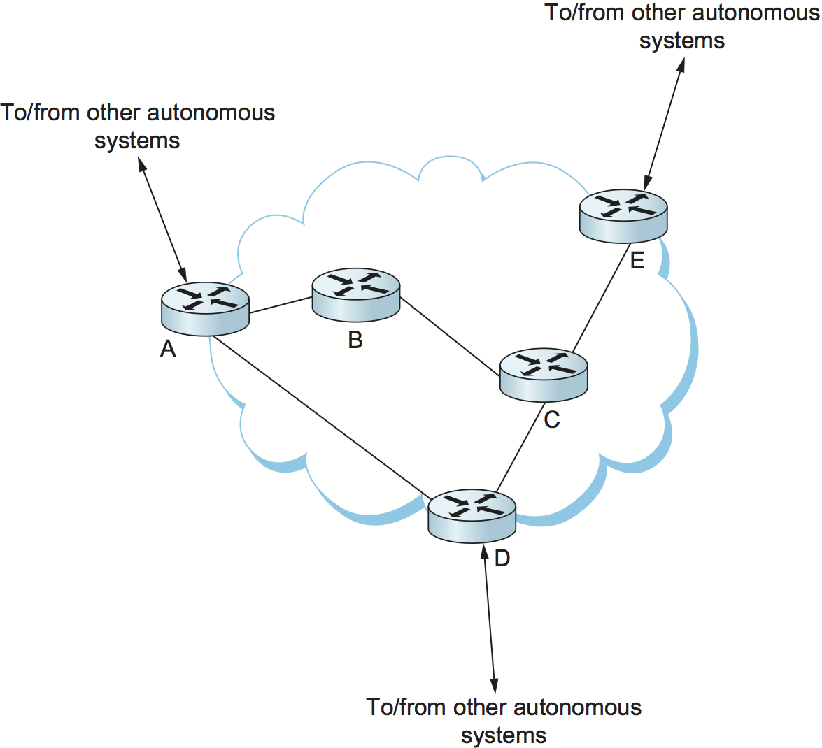
At the beginning of this chapter, we introduced the notion that the Internet is organized as autonomous systems, each of which is under the control of a single administrative entity. A corporation's complex internal network might be a single AS, as may the national network of any single Internet Service Provider (ISP). Figure 3 shows a simple network with two autonomous systems.

The basic idea behind autonomous systems is to provide an additional way to hierarchically aggregate routing information in a large internet, thus improving scalability. We now divide the routing problem into two parts: routing within a single autonomous system and routing between autonomous systems. Since another name for autonomous systems in the Internet is routing domains, we refer to the two parts of the routing problem as interdomain routing and intradomain routing. In addition to improving scalability, the AS model decouples the intradomain routing that takes place in one AS from that taking place in another. Thus, each AS can run whatever intradomain routing protocols it chooses. It can even use static routes or multiple protocols, if desired. The interdomain routing problem is then one of having different ASs share reachability information—descriptions of the set of IP addresses that can be reached via a given AS—with each other.

Challenges in Interdomain Routing

Perhaps the most important challenge of interdomain routing today is the need for each AS to determine its own routing policies. A simple example routing policy implemented at a particular AS might look like this: "Whenever possible, I prefer to send traffic via AS X than via AS Y, but I'll use AS Y if it is the only path, and I never want to carry traffic from AS X to AS Y or vice versa." Such a policy would be typical when I have paid money to both AS X and AS Y to connect my AS to the rest of the Internet, and AS X is my preferred provider of connectivity, with AS Y being the fallback. Because I view both AS X and AS Y as providers (and presumably I paid them to play this role), I don't expect to help them out by carrying traffic between them across my network (this is called transit traffic). The more autonomous systems I connect to, the more complex policies I might have, especially when you consider backbone providers, who may interconnect with dozens of other providers and hundreds of customers and have different economic arrangements (which affect routing policies) with each one.

A key design goal of interdomain routing is that policies like the example above, and much more complex ones, should be supported by the interdomain routing system. To make the problem harder, I need to be able to implement such a policy without any help from other autonomous systems, and in the face of possible misconfiguration or malicious behavior by other autonomous systems. Furthermore, there is often a desire to keep the policies private, because the entities that run the autonomous systems—mostly ISPs—are often in competition with each other and don't want their economic arrangements made public.

There have been two major interdomain routing protocols in the history of the Internet. The first was the Exterior Gateway Protocol (EGP), which had a number of limitations, perhaps the most severe of which was that it constrained the topology of the Internet rather significantly. EGP was designed when the Internet had a treelike topology, such as that illustrated in Figure 1, and did not allow for the topology to become more general. Note that in this simple treelike structure there is a single backbone, and autonomous systems are connected only as parents and children and not as peers.

The replacement for EGP was the Border Gateway Protocol (BGP), which has iterated through four versions (BGP-4). BGP is often regarded as one of the more complex parts of the Internet. We'll cover some of its high points here.

Unlike its predecessor EGP, BGP makes virtually no assumptions about how autonomous systems are interconnected—they form an arbitrary graph. This model is clearly general enough to accommodate non-tree-structured internetworks, like the simplified picture of a multi-provider Internet shown in Figure 4. (It turns out there is still some sort of structure to the Internet, as we'll see below, but it's nothing like as simple as a tree, and BGP makes no assumptions about such structure.)

Unlike the simple tree-structured Internet shown in Figure 1, or even the fairly simple picture in Figure 4, today's Internet consists of a richly interconnected set of networks, mostly operated by private companies (ISPs) rather than governments. Many Internet Service Providers (ISPs) exist mainly to provide service to "consumers" (i.e., individuals with computers in their homes), while others offer something more like the old backbone service, interconnecting other providers and sometimes larger corporations. Often, many providers arrange to interconnect with each other at a single peering point.

To get a better sense of how we might manage routing among this complex interconnection of autonomous systems, we can start by defining a few terms. We define local traffic as traffic that originates at or terminates on nodes within an AS, and transit traffic as traffic that passes through an AS. We can classify autonomous systems into three broad types:

Stub AS—an AS that has only a single connection to one other AS; such an AS will only carry local traffic. The small corporation in Figure 4 is an example of a stub AS.
Multihomed AS—an AS that has connections to more than one other AS but that refuses to carry transit traffic, such as the large corporation at the top of Figure 4.
Transit AS—an AS that has connections to more than one other AS and that is designed to carry both transit and local traffic, such as the backbone providers in Figure 4.

Whereas the discussion of routing in the previous chapter focused on finding optimal paths based on minimizing some sort of link metric, the goals of interdomain routing are rather more complex. First, it is necessary to find some path to the intended destination that is loop free. Second, paths must be compliant with the policies of the various autonomous systems along the path—and, as we have already seen, those policies might be almost arbitrarily complex. Thus, while intradomain focuses on a well-defined problem of optimizing the scalar cost of the path, interdomain focuses on finding a non-looping, policy-compliant path—a much more complex optimization problem.

There are additional factors that make interdomain routing hard. The first is simply a matter of scale. An Internet backbone router must be able to forward any packet destined anywhere in the Internet. That means having a routing table that will provide a match for any valid IP address. While CIDR has helped to control the number of distinct prefixes that are carried in the Internet's backbone routing, there is inevitably a lot of routing information to pass around—roughly 700,000 prefixes in mid-2018.

A further challenge in interdomain routing arises from the autonomous nature of the domains. Note that each domain may run its own interior routing protocols and use any scheme it chooses to assign metrics to paths. This means that it is impossible to calculate meaningful path costs for a path that crosses multiple autonomous systems. A cost of 1000 across one provider might imply a great path, but it might mean an unacceptably bad one from another provider. As a result, interdomain routing advertises only reachability. The concept of reachability is basically a statement that "you can reach this network through this AS." This means that for interdomain routing to pick an optimal path is essentially impossible.

The autonomous nature of interdomain raises issue of trust. Provider A might be unwilling to believe certain advertisements from provider B for fear that provider B will advertise erroneous routing information. For example, trusting provider B when he advertises a great route to anywhere in the Internet can be a disastrous choice if provider B turns out to have made a mistake configuring his routers or to have insufficient capacity to carry the traffic.

The issue of trust is also related to the need to support complex policies as noted above. For example, I might be willing to trust a particular provider only when he advertises reachability to certain prefixes, and thus I would have a policy that says, "Use AS X to reach only prefixes $p$ and $q$, if and only if AS X advertises reachability to those prefixes."

Basics of BGP

Each AS has one or more border routers through which packets enter and leave the AS. In our simple example in Figure 3, routers R2 and R4 would be border routers. (Over the years, routers have sometimes also been known as gateways, hence the names of the protocols BGP and EGP). A border router is simply an IP router that is charged with the task of forwarding packets between autonomous systems.

Each AS that participates in BGP must also have at least one BGP speaker, a router that "speaks" BGP to other BGP speakers in other autonomous systems. It is common to find that border routers are also BGP speakers, but that does not have to be the case.

BGP does not belong to either of the two main classes of routing protocols, distance-vector or link-state. Unlike these protocols, BGP advertises complete paths as an enumerated list of autonomous systems to reach a particular network. It is sometimes called a path-vector protocol for this reason. The advertisement of complete paths is necessary to enable the sorts of policy decisions described above to be made in accordance with the wishes of a particular AS. It also enables routing loops to be readily detected.

To see how this works, consider the very simple example network in Figure 5. Assume that the providers are transit networks, while the customer networks are stubs. A BGP speaker for the AS of provider A (AS 2) would be able to advertise reachability information for each of the network numbers assigned to customers P and Q. Thus, it would say, in effect, "The networks 128.96, 192.4.153, 192.4.32, and 192.4.3 can be reached directly from AS 2." The backbone network, on receiving this advertisement, can advertise, "The networks 128.96, 192.4.153, 192.4.32, and 192.4.3 can be reached along the path (AS 1, AS 2)." Similarly, it could advertise, "The networks 192.12.69, 192.4.54, and 192.4.23 can be reached along the path (AS 1, AS 3)."

Example of loop among autonomous systems.

An important job of BGP is to prevent the establishment of looping paths. For example, consider the network illustrated in Figure 6. It differs from Figure 5 only in the addition of an extra link between AS 2 and AS 3, but the effect now is that the graph of autonomous systems has a loop in it. Suppose AS 1 learns that it can reach network 128.96 through AS 2, so it advertises this fact to AS 3, who in turn advertises it back to AS 2. In the absence of any loop prevention mechanism, AS 2 could now decide that AS 3 was the preferred route for packets destined for 128.96. If AS 2 starts sending packets addressed to 128.96 to AS 3, AS 3 would send them to AS 1; AS 1 would send them back to AS 2; and they would loop forever. This is prevented by carrying the complete AS path in the routing messages. In this case, the advertisement for a path to 128.96 received by AS 2 from AS 3 would contain an AS path of (AS 3, AS 1, AS 2, AS 4). AS 2 sees itself in this path, and thus concludes that this is not a useful path for it to use.

In order for this loop prevention technique to work, the AS numbers carried in BGP clearly need to be unique. For example, AS 2 can only recognize itself in the AS path in the above example if no other AS identifies itself in the same way. AS numbers are now 32-bits long, and they are assigned by a central authority to assure uniqueness.

A given AS will only advertise routes that it considers good enough for itself. That is, if a BGP speaker has a choice of several different routes to a destination, it will choose the best one according to its own local policies, and then that will be the route it advertises. Furthermore, a BGP speaker is under no obligation to advertise any route to a destination, even if it has one. This is how an AS can implement a policy of not providing transit—by refusing to advertise routes to prefixes that are not contained within that AS, even if it knows how to reach them.

Given that links fail and policies change, BGP speakers need to be able to cancel previously advertised paths. This is done with a form of negative advertisement known as a withdrawn route. Both positive and negative reachability information are carried in a BGP update message, the format of which is shown in Figure 7. (Note that the fields in this figure are multiples of 16 bits, unlike other packet formats in this chapter.)

Unlike the routing protocols described in the previous chapter, BGP is defined to run on top of TCP, the reliable transport protocol. Because BGP speakers can count on TCP to be reliable, this means that any information that has been sent from one speaker to another does not need to be sent again. Thus, as long as nothing has changed, a BGP speaker can simply send an occasional keepalive message that says, in effect, "I'm still here and nothing has changed." If that router were to crash or become disconnected from its peer, it would stop sending the keepalives, and the other routers that had learned routes from it would assume that those routes were no longer valid.

Common AS Relationships and Policies

Having said that policies may be arbitrarily complex, there turn out to be a few common ones, reflecting common relationships between autonomous systems. The most common relationships are illustrated in Figure 8. The three common relationships and the policies that go with them are as follows:

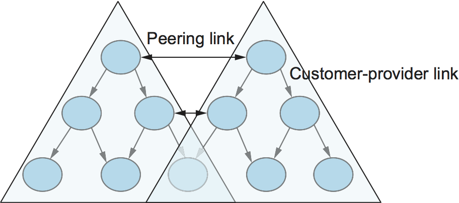
Provider-Customer—Providers are in the business of connecting their customers to the rest of the Internet. A customer might be a corporation, or it might be a smaller ISP (which may have customers of its own). So the common policy is to advertise all the routes I know about to my customer, and advertise routes I learn from my customer to everyone.
Customer-Provider—In the other direction, the customer wants to get traffic directed to him (and his customers, if he has them) by his provider, and he wants to be able to send traffic to the rest of the Internet through his provider. So the common policy in this case is to advertise my own prefixes and routes learned from my customers to my provider, advertise routes learned from my provider to my customers, but don't advertise routes learned from one provider to another provider. That last part is to make sure the customer doesn't find himself in the business of carrying traffic from one provider to another, which isn't in his interests if he is paying the providers to carry traffic for him.
Peer—The third option is a symmetrical peering between autonomous systems. Two providers who view themselves as equals usually peer so that they can get access to each other's customers without having to pay another provider. The typical policy here is to advertise routes learned from my customers to my peer, advertise routes learned from my peer to my customers, but don't advertise routes from my peer to any provider or vice versa.

One thing to note about this figure is the way it has brought back some structure to the apparently unstructured Internet. At the bottom of the hierarchy we have the stub networks that are customers of one or more providers, and as we move up the hierarchy we see providers who have other providers as their customers. At the top, we have providers who have customers and peers but are not customers of anyone. These providers are known as the Tier-1 providers.

Key Takeaway

Let's return to the real question: How does all this help us to build scalable networks? First, the number of nodes participating in BGP is on the order of the number of autonomous systems, which is much smaller than the number of networks. Second, finding a good interdomain route is only a matter of finding a path to the right border router, of which there are only a few per AS. Thus, we have neatly subdivided the routing problem into manageable parts, once again using a new level of hierarchy to increase scalability. The complexity of interdomain routing is now on the order of the number of autonomous systems, and the complexity of intradomain routing is on the order of the number of networks in a single AS.

Integrating Interdomain and Intradomain Routing

While the preceding discussion illustrates how a BGP speaker learns interdomain routing information, the question still remains as to how all the other routers in a domain get this information. There are several ways this problem can be addressed.

Let's start with a very simple situation, which is also very common. In the case of a stub AS that only connects to other autonomous systems at a single point, the border router is clearly the only choice for all routes that are outside the AS. Such a router can inject a default route into the intradomain routing protocol. In effect, this is a statement that any network that has not been explicitly advertised in the intradomain protocol is reachable through the border router. Recall from the discussion of IP forwarding in the previous chapter that the default entry in the forwarding table comes after all the more specific entries, and it matches anything that failed to match a specific entry.

The next step up in complexity is to have the border routers inject specific routes they have learned from outside the AS. Consider, for example, the border router of a provider AS that connects to a customer AS. That router could learn that the network prefix 192.4.54/24 is located inside the customer AS, either through BGP or because the information is configured into the border router. It could inject a route to that prefix into the routing protocol running inside the provider AS. This would be an advertisement of the sort, "I have a link to 192.4.54/24 of cost X." This would cause other routers in the provider AS to learn that this border router is the place to send packets destined for that prefix.

The final level of complexity comes in backbone networks, which learn so much routing information from BGP that it becomes too costly to inject it into the intradomain protocol. For example, if a border router wants to inject 10,000 prefixes that it learned about from another AS, it will have to send very big link-state packets to the other routers in that AS, and their shortest-path calculations are going to become very complex. For this reason, the routers in a backbone network use a variant of BGP called interior BGP (iBGP) to effectively redistribute the information that is learned by the BGP speakers at the edges of the AS to all the other routers in the AS. (The other variant of BGP, discussed above, runs between autonomous systems and is called exterior BGP, or eBGP). iBGP enables any router in the AS to learn the best border router to use when sending a packet to any address. At the same time, each router in the AS keeps track of how to get to each border router using a conventional intradomain protocol with no injected information. By combining these two sets of information, each router in the AS is able to determine the appropriate next hop for all prefixes.

Example of interdomain and intradomain routing. All routers run iBGP and an intradomain routing protocol. Border routers A, D, and E also run eBGP to other autonomous systems.

To see how this all works, consider the simple example network, representing a single AS, in Figure 9. The three border routers, A, D, and E, speak eBGP to other autonomous systems and learn how to reach various prefixes. These three border routers communicate with other and with the interior routers B and C by building a mesh of iBGP sessions among all the routers in the AS. Let's now focus in on how router B builds up its complete view of how to forward packets to any prefix. Look at the top left of Figure 10, which shows the information that router B learns from its iBGP sessions. It learns that some prefixes are best reached via router A, some via D, and some via E. At the same time, all the routers in the AS are also running some intradomain routing protocol such as Routing Information Protocol (RIP) or Open Shortest Path First (OSPF). (A generic term for intradomain protocols is an interior gateway protocol, or IGP.) From this completely separate protocol, B learns how to reach other nodes inside the domain, as shown in the top right table. For example, to reach router E, B needs to send packets toward router C. Finally, in the bottom table, B puts the whole picture together, combining the information about external prefixes learned from iBGP with the information about interior routes to the border routers learned from the IGP. Thus, if a prefix like 18.0/16 is reachable via border router E, and the best interior path to E is via C, then it follows that any packet destined for 18.0/16 should be forwarded toward C. In this way, any router in the AS can build up a complete routing table for any prefix that is reachable via some border router of the AS.

BGP routing table, IGP routing table, and combined table at router B.

IP Version 6 (IPv6)

In many respects, the motivation for a new version of IP is simple: to deal with exhaustion of the IP address space. CIDR helped considerably to contain the rate at which the Internet address space is being consumed and also helped to control the growth of routing table information needed in the Internet's routers. However, there will come a point at which these techniques are no longer adequate. In particular, it is virtually impossible to achieve 100% address utilization efficiency, so the address space will be exhausted well before the 4 billionth host is connected to the Internet. Even if we were able to use all 4 billion addresses, it's not too hard to imagine ways that that number could be exhausted, now that IP addresses are assigned not just to full-blown computers but also to mobile phones, televisions, and other household appliances. All of these possibilities argue that a bigger address space than that provided by 32 bits will eventually be needed.

Historical Perspective

The IETF began looking at the problem of expanding the IP address space in 1991, and several alternatives were proposed. Since the IP address is carried in the header of every IP packet, increasing the size of the address dictates a change in the packet header. This means a new version of the Internet Protocol and, as a consequence, a need for new software for every host and router in the Internet. This is clearly not a trivial matter—it is a major change that needs to be thought about very carefully.

The effort to define a new version of IP was known as IP Next Generation, or IPng. As the work progressed, an official IP version number was assigned, so IPng is now known as IPv6. Note that the version of IP discussed so far in this chapter is version 4 (IPv4). The apparent discontinuity in numbering is the result of version number 5 being used for an experimental protocol many years ago.

The significance of changing to a new version of IP caused a snowball effect. The general feeling among network designers was that if you are going to make a change of this magnitude you might as well fix as many other things in IP as possible at the same time. Consequently, the IETF solicited white papers from anyone who cared to write one, asking for input on the features that might be desired in a new version of IP. In addition to the need to accommodate scalable routing and addressing, some of the other wish list items for IPng included:

Support for real-time services
Security support
Autoconfiguration (i.e., the ability of hosts to automatically configure themselves with such information as their own IP address and domain name)
Enhanced routing functionality, including support for mobile hosts

It is interesting to note that, while many of these features were absent from IPv4 at the time IPv6 was being designed, support for all of them has made its way into IPv4 in recent years, often using similar techniques in both protocols. It can be argued that the freedom to think of IPv6 as a clean slate facilitated the design of new capabilities for IP that were then retrofitted into IPv4.

In addition to the wish list, one absolutely non-negotiable feature for IPng was that there must be a transition plan to move from the current version of IP (version 4) to the new version. With the Internet being so large and having no centralized control, it would be completely impossible to have a "flag day" on which everyone shut down their hosts and routers and installed a new version of IP. Thus, we can expect there to be a long transition period in which some hosts and routers will run IPv4 only, some will run IPv4 and IPv6, and some will run IPv6 only. (So far, that transition period has lasted over 20 years!)

The IETF appointed a committee called the IPng Directorate to collect all the inputs on IPng requirements and to evaluate proposals for a protocol to become IPng. Over the life of this committee there were numerous proposals, some of which merged with other proposals, and eventually one was chosen by the Directorate to be the basis for IPng. That proposal was called Simple Internet Protocol Plus (SIPP). SIPP originally called for a doubling of the IP address size to 64 bits. When the Directorate selected SIPP, they stipulated several changes, one of which was another doubling of the address to 128 bits (16 bytes). It was around this time that version number 6 was assigned. The rest of this section describes some of the main features of IPv6. At the time of this writing, most of the key specifications for IPv6 are Proposed or Draft Standards in the IETF.

Addresses and Routing

First and foremost, IPv6 provides a 128-bit address space, as opposed to the 32 bits of version 4. Thus, while version 4 can potentially address 4 billion nodes if address assignment efficiency reaches 100%, IPv6 can address $3.4 \times 10^{38}$ nodes, again assuming 100% efficiency. As we have seen, though, 100% efficiency in address assignment is not likely. Some analysis of other addressing schemes, such as those of the French and U.S. telephone networks, as well as that of IPv4, have turned up some empirical numbers for address assignment efficiency. Based on the most pessimistic estimates of efficiency drawn from this study, the IPv6 address space is predicted to provide over 1500 addresses per square foot of the Earth's surface, which certainly seems like it should serve us well even when toasters on Venus have IP addresses.

Address Space Allocation

Drawing on the effectiveness of CIDR in IPv4, IPv6 addresses are also classless, but the address space is still subdivided in various ways based on the leading bits. Rather than specifying different address classes, the leading bits specify different uses of the IPv6 address. The current assignment of prefixes is listed in Table 1.

Prefix	Use
00...0 (128 bits)	Unspecified
00...1 (128 bits)	Loopback
1111 1111	Multicast addresses
1111 1110 10	Link-local unicast
Everything else	Global Unicast

This allocation of the address space warrants a little discussion. First, the entire functionality of IPv4's three main address classes (A, B, and C) is contained inside the "everything else" range. Global Unicast Addresses, as we will see shortly, are a lot like classless IPv4 addresses, only much longer. These are the main ones of interest at this point, with over 99% of the total IPv6 address space available to this important form of address. (At the time of writing, IPv6 unicast addresses are being allocated from the block that begins 001, with the remaining address space—about 87%—being reserved for future use.)

The multicast address space is (obviously) for multicast, thereby serving the same role as class D addresses in IPv4. Note that multicast addresses are easy to distinguish—they start with a byte of all 1s. We will see how these addresses are used in a later section.

The idea behind link-local use addresses is to enable a host to construct an address that will work on the network to which it is connected without being concerned about the global uniqueness of the address. This may be useful for autoconfiguration, as we will see below. Similarly, the site-local use addresses are intended to allow valid addresses to be constructed on a site (e.g., a private corporate network) that is not connected to the larger Internet; again, global uniqueness need not be an issue.

Within the global unicast address space are some important special types of addresses. A node may be assigned an IPv4-compatible IPv6 address by zero-extending a 32-bit IPv4 address to 128 bits. A node that is only capable of understanding IPv4 can be assigned an IPv4-mapped IPv6 address by prefixing the 32-bit IPv4 address with 2 bytes of all 1s and then zero-extending the result to 128 bits. These two special address types have uses in the IPv4-to-IPv6 transition (see the sidebar on this topic).

Address Notation

Just as with IPv4, there is some special notation for writing down IPv6 addresses. The standard representation is x:x:x:x:x:x:x:x, where each x is a hexadecimal representation of a 16-bit piece of the address. An example would be

47CD:1234:4422:ACO2:0022:1234:A456:0124

Any IPv6 address can be written using this notation. Since there are a few special types of IPv6 addresses, there are some special notations that may be helpful in certain circumstances. For example, an address with a large number of contiguous 0s can be written more compactly by omitting all the 0 fields. Thus,

47CD:0000:0000:0000:0000:0000:A456:0124

could be written

47CD::A456:0124

Clearly, this form of shorthand can only be used for one set of contiguous 0s in an address to avoid ambiguity.

The two types of IPv6 addresses that contain an embedded IPv4 address have their own special notation that makes extraction of the IPv4 address easier. For example, the IPv4-mapped IPv6 address of a host whose IPv4 address was 128.96.33.81 could be written as

::FFFF:128.96.33.81

That is, the last 32 bits are written in IPv4 notation, rather than as a pair of hexadecimal numbers separated by a colon. Note that the double colon at the front indicates the leading 0s.

Global Unicast Addresses

By far the most important sort of addressing that IPv6 must provide is plain old unicast addressing. It must do this in a way that supports the rapid rate of addition of new hosts to the Internet and that allows routing to be done in a scalable way as the number of physical networks in the Internet grows. Thus, at the heart of IPv6 is the unicast address allocation plan that determines how unicast addresses will be assigned to service providers, autonomous systems, networks, hosts, and routers.

In fact, the address allocation plan that is proposed for IPv6 unicast addresses is extremely similar to that being deployed with CIDR in IPv4. To understand how it works and how it provides scalability, it is helpful to define some new terms. We may think of a nontransit AS (i.e., a stub or multihomed AS) as a subscriber, and we may think of a transit AS as a provider. Furthermore, we may subdivide providers into direct and indirect. The former are directly connected to subscribers. The latter primarily connect other providers, are not connected directly to subscribers, and are often known as backbone networks.

With this set of definitions, we can see that the Internet is not just an arbitrarily interconnected set of autonomous systems; it has some intrinsic hierarchy. The difficulty lies in making use of this hierarchy without inventing mechanisms that fail when the hierarchy is not strictly observed, as happened with EGP. For example, the distinction between direct and indirect providers becomes blurred when a subscriber connects to a backbone or when a direct provider starts connecting to many other providers.

As with CIDR, the goal of the IPv6 address allocation plan is to provide aggregation of routing information to reduce the burden on intradomain routers. Again, the key idea is to use an address prefix—a set of contiguous bits at the most significant end of the address—to aggregate reachability information to a large number of networks and even to a large number of autonomous systems. The main way to achieve this is to assign an address prefix to a direct provider and then for that direct provider to assign longer prefixes that begin with that prefix to its subscribers. Thus, a provider can advertise a single prefix for all of its subscribers.

Of course, the drawback is that if a site decides to change providers, it will need to obtain a new address prefix and renumber all the nodes in the site. This could be a colossal undertaking, enough to dissuade most people from ever changing providers. For this reason, there is ongoing research on other addressing schemes, such as geographic addressing, in which a site's address is a function of its location rather than the provider to which it attaches. At present, however, provider-based addressing is necessary to make routing work efficiently.

Note that while IPv6 address assignment is essentially equivalent to the way address assignment has happened in IPv4 since the introduction of CIDR, IPv6 has the significant advantage of not having a large installed base of assigned addresses to fit into its plans.

One question is whether it makes sense for hierarchical aggregation to take place at other levels in the hierarchy. For example, should all providers obtain their address prefixes from within a prefix allocated to the backbone to which they connect? Given that most providers connect to multiple backbones, this probably doesn't make sense. Also, since the number of providers is much smaller than the number of sites, the benefits of aggregating at this level are much fewer.

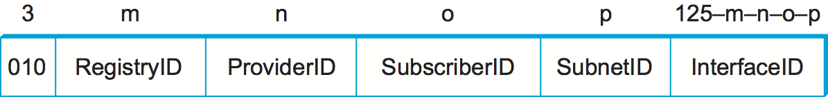
One place where aggregation may make sense is at the national or continental level. Continental boundaries form natural divisions in the Internet topology. If all addresses in Europe, for example, had a common prefix, then a great deal of aggregation could be done, and most routers in other continents would only need one routing table entry for all networks with the Europe prefix. Providers in Europe would all select their prefixes such that they began with the European prefix. Using this scheme, an IPv6 address might look like Figure 11. The RegistryID might be an identifier assigned to a European address registry, with different IDs assigned to other continents or countries. Note that prefixes would be of different lengths under this scenario. For example, a provider with few customers could have a longer prefix (and thus less total address space available) than one with many customers.

One tricky situation could occur when a subscriber is connected to more than one provider. Which prefix should the subscriber use for his or her site? There is no perfect solution to the problem. For example, suppose a subscriber is connected to two providers, X and Y. If the subscriber takes his prefix from X, then Y has to advertise a prefix that has no relationship to its other subscribers and that as a consequence cannot be aggregated. If the subscriber numbers part of his AS with the prefix of X and part with the prefix of Y, he runs the risk of having half his site become unreachable if the connection to one provider goes down. One solution that works fairly well if X and Y have a lot of subscribers in common is for them to have three prefixes between them: one for subscribers of X only, one for subscribers of Y only, and one for the sites that are subscribers of both X and Y.

Packet Format

Despite the fact that IPv6 extends IPv4 in several ways, its header format is actually simpler. This simplicity is due to a concerted effort to remove unnecessary functionality from the protocol. Figure 12 shows the result.

As with many headers, this one starts with a Version field, which is set to 6 for IPv6. The Version field is in the same place relative to the start of the header as IPv4's Version field so that header-processing software can immediately decide which header format to look for. The TrafficClass and FlowLabel fields both relate to quality of service issues.

The PayloadLen field gives the length of the packet, excluding the IPv6 header, measured in bytes. The NextHeader field cleverly replaces both the IP options and the Protocol field of IPv4. If options are required, then they are carried in one or more special headers following the IP header, and this is indicated by the value of the NextHeader field. If there are no special headers, the NextHeader field is the demux key identifying the higher-level protocol running over IP (e.g., TCP or UDP); that is, it serves the same purpose as the IPv4 Protocol field. Also, fragmentation is now handled as an optional header, which means that the fragmentation-related fields of IPv4 are not included in the IPv6 header. The HopLimit field is simply the TTL of IPv4, renamed to reflect the way it is actually used.

Finally, the bulk of the header is taken up with the source and destination addresses, each of which is 16 bytes (128 bits) long. Thus, the IPv6 header is always 40 bytes long. Considering that IPv6 addresses are four times longer than those of IPv4, this compares quite well with the IPv4 header, which is 20 bytes long in the absence of options.

The way that IPv6 handles options is quite an improvement over IPv4. In IPv4, if any options were present, every router had to parse the entire options field to see if any of the options were relevant. This is because the options were all buried at the end of the IP header, as an unordered collection of '(type, length, value)' tuples. In contrast, IPv6 treats options as extension headers that must, if present, appear in a specific order. This means that each router can quickly determine if any of the options are relevant to it; in most cases, they will not be. Usually this can be determined by just looking at the NextHeader field. The end result is that option processing is much more efficient in IPv6, which is an important factor in router performance. In addition, the new formatting of options as extension headers means that they can be of arbitrary length, whereas in IPv4 they were limited to 44 bytes at most. We will see how some of the options are used below.

Each option has its own type of extension header. The type of each extension header is identified by the value of the NextHeader field in the header that precedes it, and each extension header contains a NextHeader field to identify the header following it. The last extension header will be followed by a transport-layer header (e.g., TCP) and in this case the value of the NextHeader field is the same as the value of the Protocol field would be in an IPv4 header. Thus, the NextHeader field does double duty; it may either identify the type of extension header to follow, or, in the last extension header, it serves as a demux key to identify the higher-layer protocol running over IPv6.

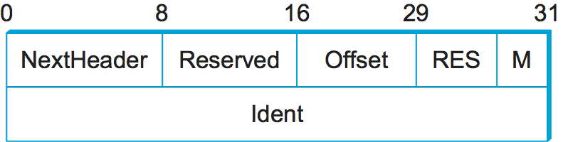
Consider the example of the fragmentation header, shown in Figure 13. This header provides functionality similar to the fragmentation fields in the IPv4 header, but it is only present if fragmentation is necessary. Assuming it is the only extension header present, then the NextHeader field of the IPv6 header would contain the value 44, which is the value assigned to indicate the fragmentation header. The NextHeader field of the fragmentation header itself contains a value describing the header that follows it. Again, assuming no other extension headers are present, then the next header might be the TCP header, which results in NextHeader containing the value 6, just as the Protocol field would in IPv4. If the fragmentation header were followed by, say, an authentication header, then the fragmentation header's NextHeader field would contain the value 51.

Autoconfiguration

While the Internet's growth has been impressive, one factor that has inhibited faster acceptance of the technology is the fact that getting connected to the Internet has typically required a fair amount of system administration expertise. In particular, every host that is connected to the Internet needs to be configured with a certain minimum amount of information, such as a valid IP address, a subnet mask for the link to which it attaches, and the address of a name server. Thus, it has not been possible to unpack a new computer and connect it to the Internet without some preconfiguration. One goal of IPv6, therefore, is to provide support for autoconfiguration, sometimes referred to as plug-and-play operation.

As we saw in the previous chapter, autoconfiguration is possible for IPv4, but it depends on the existence of a server that is configured to hand out addresses and other configuration information to Dynamic Host Configuration Protocol (DHCP) clients. The longer address format in IPv6 helps provide a useful, new form of autoconfiguration called stateless autoconfiguration, which does not require a server.

Recall that IPv6 unicast addresses are hierarchical, and that the least significant portion is the interface ID. Thus, we can subdivide the autoconfiguration problem into two parts:

Obtain an interface ID that is unique on the link to which the host is attached.
Obtain the correct address prefix for this subnet.

The first part turns out to be rather easy, since every host on a link must have a unique link-level address. For example, all hosts on an Ethernet have a unique 48-bit Ethernet address. This can be turned into a valid link-local use address by adding the appropriate prefix from Table (1111 1110 10) followed by enough 0s to make up 128 bits. For some devices—for example, printers or hosts on a small routerless network that do not connect to any other networks—this address may be perfectly adequate. Those devices that need a globally valid address depend on a router on the same link to periodically advertise the appropriate prefix for the link. Clearly, this requires that the router be configured with the correct address prefix, and that this prefix be chosen in such a way that there is enough space at the end (e.g., 48 bits) to attach an appropriate link-level address.

The ability to embed link-level addresses as long as 48 bits into IPv6 addresses was one of the reasons for choosing such a large address size. Not only does 128 bits allow the embedding, but it leaves plenty of space for the multilevel hierarchy of addressing that we discussed above.

Advanced Routing Capabilities

Another of IPv6's extension headers is the routing header. In the absence of this header, routing for IPv6 differs very little from that of IPv4 under CIDR. The routing header contains a list of IPv6 addresses that represent nodes or topological areas that the packet should visit en route to its destination. A topological area may be, for example, a backbone provider's network. Specifying that packets must visit this network would be a way of implementing provider selection on a packet-by-packet basis. Thus, a host could say that it wants some packets to go through a provider that is cheap, others through a provider that provides high reliability, and still others through a provider that the host trusts to provide security.

To provide the ability to specify topological entities rather than individual nodes, IPv6 defines an anycast address. An anycast address is assigned to a set of interfaces, and packets sent to that address will go to the "nearest" of those interfaces, with nearest being determined by the routing protocols. For example, all the routers of a backbone provider could be assigned a single anycast address, which would be used in the routing header.

The anycast address and the routing header are also expected to be used to provide enhanced routing support to mobile hosts. The detailed mechanisms for providing this support are still being defined.

Other Features

As mentioned at the beginning of this section, the primary motivation behind the development of IPv6 was to support the continued growth of the Internet. Once the IP header had to be changed for the sake of the addresses, however, the door was open for a wide variety of other changes, two of which we have just described—autoconfiguration and source-directed routing. IPv6 includes several additional features, most of which are covered elsewhere in this book; e.g., mobility, security, quality-of-service. It is interesting to note that, in most of these areas, the IPv4 and IPv6 capabilities have become virtually indistinguishable, so that the main driver for IPv6 remains the need for larger addresses.