3.4: Loop Optimizations

Introduction

In nearly all high performance applications, loops are where the majority of the execution time is spent. In [Section 2.3] we examined ways in which application developers introduced clutter into loops, possibly slowing those loops down. In this chapter we focus on techniques used to improve the performance of these “clutter-free” loops. Sometimes the compiler is clever enough to generate the faster versions of the loops, and other times we have to do some rewriting of the loops ourselves to help the compiler.

It’s important to remember that one compiler’s performance enhancing modifications are another compiler’s clutter. When you make modifications in the name of performance you must make sure you’re helping by testing the performance with and without the modifications. Also, when you move to another architecture you need to make sure that any modifications aren’t hindering performance. For this reason, you should choose your performance-related modifications wisely. You should also keep the original (simple) version of the code for testing on new architectures. Also if the benefit of the modification is small, you should probably keep the code in its most simple and clear form.

We look at a number of different loop optimization techniques, including:

• Loop unrolling
• Nested loop optimization
• Loop interchange
• Memory reference optimization
• Blocking
• Out-of-core solutions

Someday, it may be possible for a compiler to perform all these loop optimizations automatically. Typically loop unrolling is performed as part of the normal compiler optimizations. Other optimizations may have to be triggered using explicit compile-time options. As you contemplate making manual changes, look carefully at which of these optimizations can be done by the compiler. Also run some tests to determine if the compiler optimizations are as good as hand optimizations.

Operation Counting

Before you begin to rewrite a loop body or reorganize the order of the loops, you must have some idea of what the body of the loop does for each iteration. Operation counting is the process of surveying a loop to understand the operation mix. You need to count the number of loads, stores, floating-point, integer, and library calls per iteration of the loop. From the count, you can see how well the operation mix of a given loop matches the capabilities of the processor. Of course, operation counting doesn’t guarantee that the compiler will generate an efficient representation of a loop.¹ But it generally provides enough insight to the loop to direct tuning efforts.

Bear in mind that an instruction mix that is balanced for one machine may be imbalanced for another. Processors on the market today can generally issue some combination of one to four operations per clock cycle. Address arithmetic is often embedded in the instructions that reference memory. Because the compiler can replace complicated loop address calculations with simple expressions (provided the pattern of addresses is predictable), you can often ignore address arithmetic when counting operations.²

Let’s look at a few loops and see what we can learn about the instruction mix:

      DO I=1,N
        A(I,J,K) = A(I,J,K) + B(J,I,K)
      ENDDO

This loop contains one floating-point addition and three memory references (two loads and a store). There are some complicated array index expressions, but these will probably be simplified by the compiler and executed in the same cycle as the memory and floating-point operations. For each iteration of the loop, we must increment the index variable and test to determine if the loop has completed.

A 3:1 ratio of memory references to floating-point operations suggests that we can hope for no more than 1/3 peak floating-point performance from the loop unless we have more than one path to memory. That’s bad news, but good information. The ratio tells us that we ought to consider memory reference optimizations first.

The loop below contains one floating-point addition and two memory operations — a load and a store. Operand B(J) is loop-invariant, so its value only needs to be loaded once, upon entry to the loop:

      DO I=1,N
        A(I) = A(I) + B(J)
      ENDDO

Again, our floating-point throughput is limited, though not as severely as in the previous loop. The ratio of memory references to floating-point operations is 2:1.

The next example shows a loop with better prospects. It performs element-wise multiplication of two vectors of complex numbers and assigns the results back to the first. There are six memory operations (four loads and two stores) and six floating-point operations (two additions and four multiplications):

      for (i=0; i<n; i++) {
          xr[i] = xr[i] * yr[i] - xi[i] * yi[i];
          xi[i] = xr[i] * yi[i] + xi[i] * yr[i];
      }

It appears that this loop is roughly balanced for a processor that can perform the same number of memory operations and floating-point operations per cycle. However, it might not be. Many processors perform a floating-point multiply and add in a single instruction. If the compiler is good enough to recognize that the multiply-add is appropriate, this loop may also be limited by memory references; each iteration would be compiled into two multiplications and two multiply-adds.

Again, operation counting is a simple way to estimate how well the requirements of a loop will map onto the capabilities of the machine. For many loops, you often find the performance of the loops dominated by memory references, as we have seen in the last three examples. This suggests that memory reference tuning is very important.

Basic Loop Unrolling

The most basic form of loop optimization is loop unrolling. It is so basic that most of today’s compilers do it automatically if it looks like there’s a benefit. There has been a great deal of clutter introduced into old dusty-deck FORTRAN programs in the name of loop unrolling that now serves only to confuse and mislead today’s compilers.

We’re not suggesting that you unroll any loops by hand. The purpose of this section is twofold. First, once you are familiar with loop unrolling, you might recognize code that was unrolled by a programmer (not you) some time ago and simplify the code. Second, you need to understand the concepts of loop unrolling so that when you look at generated machine code, you recognize unrolled loops.

The primary benefit in loop unrolling is to perform more computations per iteration. At the end of each iteration, the index value must be incremented, tested, and the control is branched back to the top of the loop if the loop has more iterations to process. By unrolling the loop, there are less “loop-ends” per loop execution. Unrolling also reduces the overall number of branches significantly and gives the processor more instructions between branches (i.e., it increases the size of the basic blocks).

For illustration, consider the following loop. It has a single statement wrapped in a do-loop:

      DO I=1,N
        A(I) = A(I) + B(I) * C
      ENDDO

You can unroll the loop, as we have below, giving you the same operations in fewer iterations with less loop overhead. You can imagine how this would help on any computer. Because the computations in one iteration do not depend on the computations in other iterations, calculations from different iterations can be executed together. On a superscalar processor, portions of these four statements may actually execute in parallel:

      DO I=1,N,4
        A(I) = A(I) + B(I) * C
        A(I+1) = A(I+1) + B(I+1) * C
        A(I+2) = A(I+2) + B(I+2) * C
        A(I+3) = A(I+3) + B(I+3) * C
      ENDDO

However, this loop is not exactly the same as the previous loop. The loop is unrolled four times, but what if N is not divisible by 4? If not, there will be one, two, or three spare iterations that don’t get executed. To handle these extra iterations, we add another little loop to soak them up. The extra loop is called a preconditioning loop:

      II = IMOD (N,4)
      DO I=1,II
        A(I) = A(I) + B(I) * C
      ENDDO

      DO I=1+II,N,4
        A(I)   = A(I) + B(I) * C
        A(I+1) = A(I+1) + B(I+1) * C
        A(I+2) = A(I+2) + B(I+2) * C
        A(I+3) = A(I+3) + B(I+3) * C
      ENDDO

The number of iterations needed in the preconditioning loop is the total iteration count modulo for this unrolling amount. If, at runtime, N turns out to be divisible by 4, there are no spare iterations, and the preconditioning loop isn’t executed.

Speculative execution in the post-RISC architecture can reduce or eliminate the need for unrolling a loop that will operate on values that must be retrieved from main memory. Because the load operations take such a long time relative to the computations, the loop is naturally unrolled. While the processor is waiting for the first load to finish, it may speculatively execute three to four iterations of the loop ahead of the first load, effectively unrolling the loop in the Instruction Reorder Buffer.

Qualifying Candidates for Loop Unrolling Up one level

Assuming a large value for N, the previous loop was an ideal candidate for loop unrolling. The iterations could be executed in any order, and the loop innards were small. But as you might suspect, this isn’t always the case; some kinds of loops can’t be unrolled so easily. Additionally, the way a loop is used when the program runs can disqualify it for loop unrolling, even if it looks promising.

In this section we are going to discuss a few categories of loops that are generally not prime candidates for unrolling, and give you some ideas of what you can do about them. We talked about several of these in the previous chapter as well, but they are also relevant here.

Loops with Low Trip Counts

To be effective, loop unrolling requires a fairly large number of iterations in the original loop. To understand why, picture what happens if the total iteration count is low, perhaps less than 10, or even less than 4. With a trip count this low, the preconditioning loop is doing a proportionately large amount of the work. It’s not supposed to be that way. The preconditioning loop is supposed to catch the few leftover iterations missed by the unrolled, main loop. However, when the trip count is low, you make one or two passes through the unrolled loop, plus one or two passes through the preconditioning loop. In other words, you have more clutter; the loop shouldn’t have been unrolled in the first place.

Probably the only time it makes sense to unroll a loop with a low trip count is when the number of iterations is constant and known at compile time. For instance, suppose you had the following loop:

      PARAMETER (NITER = 3)
      DO I=1,NITER
        A(I) = B(I) * C
      ENDDO

Because NITER is hardwired to 3, you can safely unroll to a depth of 3 without worrying about a preconditioning loop. In fact, you can throw out the loop structure altogether and leave just the unrolled loop innards:

      PARAMETER (NITER = 3)
      A(1) = B(1) * C
      A(2) = B(2) * C
      A(3) = A(3) * C

Of course, if a loop’s trip count is low, it probably won’t contribute significantly to the overall runtime, unless you find such a loop at the center of a larger loop. Then you either want to unroll it completely or leave it alone.

Fat Loops

Loop unrolling helps performance because it fattens up a loop with more calculations per iteration. By the same token, if a particular loop is already fat, unrolling isn’t going to help. The loop overhead is already spread over a fair number of instructions. In fact, unrolling a fat loop may even slow your program down because it increases the size of the text segment, placing an added burden on the memory system (we’ll explain this in greater detail shortly). A good rule of thumb is to look elsewhere for performance when the loop innards exceed three or four statements.

Loops Containing Procedure Calls

As with fat loops, loops containing subroutine or function calls generally aren’t good candidates for unrolling. There are several reasons. First, they often contain a fair number of instructions already. And if the subroutine being called is fat, it makes the loop that calls it fat as well. The size of the loop may not be apparent when you look at the loop; the function call can conceal many more instructions.

Second, when the calling routine and the subroutine are compiled separately, it’s impossible for the compiler to intermix instructions. A loop that is unrolled into a series of function calls behaves much like the original loop, before unrolling.

Last, function call overhead is expensive. Registers have to be saved; argument lists have to be prepared. The time spent calling and returning from a subroutine can be much greater than that of the loop overhead. Unrolling to amortize the cost of the loop structure over several calls doesn’t buy you enough to be worth the effort.

The general rule when dealing with procedures is to first try to eliminate them in the “remove clutter” phase, and when this has been done, check to see if unrolling gives an additional performance improvement.

Loops with Branches in Them

In [Section 2.3] we showed you how to eliminate certain types of branches, but of course, we couldn’t get rid of them all. In cases of iteration-independent branches, there might be some benefit to loop unrolling. The IF test becomes part of the operations that must be counted to determine the value of loop unrolling. Below is a doubly nested loop. The inner loop tests the value of B(J,I):

      DO I=1,N
        DO J=1,N
          IF (B(J,I) .GT. 1.0) A(J,I) = A(J,I) + B(J,I) * C
        ENDDO
      ENDDO

Each iteration is independent of every other, so unrolling it won’t be a problem. We’ll just leave the outer loop undisturbed:

      II = IMOD (N,4)
      DO I=1,N
        DO J=1,II
          IF (B(J,I) .GT. 1.0)
      +     A(J,I) = A(J,I) + B(J,I) * C
          ENDDO
          DO J=II+1,N,4
            IF (B(J,I) .GT. 1.0)
      +       A(J,I) = A(J,I) + B(J,I) * C
            IF (B(J+1,I) .GT. 1.0)
      +       A(J+1,I) = A(J+1,I) + B(J+1,I) * C
            IF (B(J+2,I) .GT. 1.0)
      +       A(J+2,I) = A(J+2,I) + B(J+2,I) * C
            IF (B(J+3,I) .GT. 1.0)
      +       A(J+3,I) = A(J+3,I) + B(J+3,I) * C
          ENDDO
        ENDDO

This approach works particularly well if the processor you are using supports conditional execution. As described earlier, conditional execution can replace a branch and an operation with a single conditionally executed assignment. On a superscalar processor with conditional execution, this unrolled loop executes quite nicely.

Nested Loops

When you embed loops within other loops, you create a loop nest. The loop or loops in the center are called the inner loops. The surrounding loops are called outer loops. Depending on the construction of the loop nest, we may have some flexibility in the ordering of the loops. At times, we can swap the outer and inner loops with great benefit. In the next sections we look at some common loop nestings and the optimizations that can be performed on these loop nests.

Often when we are working with nests of loops, we are working with multidimensional arrays. Computing in multidimensional arrays can lead to non-unit-stride memory access. Many of the optimizations we perform on loop nests are meant to improve the memory access patterns.

First, we examine the computation-related optimizations followed by the memory optimizations.

Outer Loop Unrolling

If you are faced with a loop nest, one simple approach is to unroll the inner loop. Unrolling the innermost loop in a nest isn’t any different from what we saw above. You just pretend the rest of the loop nest doesn’t exist and approach it in the nor- mal way. However, there are times when you want to apply loop unrolling not just to the inner loop, but to outer loops as well — or perhaps only to the outer loops. Here’s a typical loop nest:

      for (i=0; i<n; i++)
          for (j=0; j<n; j++)
              for (k=0; k<n; k++)
                  a[i][j][k] = a[i][j][k] + b[i][j][k] * c;

To unroll an outer loop, you pick one of the outer loop index variables and replicate the innermost loop body so that several iterations are performed at the same time, just like we saw in the [Section 2.4.4]. The difference is in the index variable for which you unroll. In the code below, we have unrolled the middle (j) loop twice:

      for (i=0; i<n; i++)
          for (j=0; j<n; j+=2)
              for (k=0; k<n; k++) {
                  a[i][j][k] = a[i][j][k] + b[i][k][j] * c;
                  a[i][j+1][k] = a[i][j+1][k] + b[i][k][j+1] * c;
              }

We left the k loop untouched; however, we could unroll that one, too. That would give us outer and inner loop unrolling at the same time:

      for (i=0; i<n; i++)
          for (j=0; j<n; j+=2)
              for (k=0; k<n; k+=2) {
                  a[i][j][k]     = a[i][j][k]     + b[i][k][j] * c;
                  a[i][j+1][k]   = a[i][j+1][k]   + b[i][k][j+1] * c;
                  a[i][j][k+1]   = a[i][j][k+1]   + b[i][k+1][j] * c;
                  a[i][j+1][k+1] = a[i][j+1][k+1] + b[i][k+1][j+1] * c;
              }

We could even unroll the i loop too, leaving eight copies of the loop innards. (Notice that we completely ignored preconditioning; in a real application, of course, we couldn’t.)

Outer Loop Unrolling to Expose Computations

Say that you have a doubly nested loop and that the inner loop trip count is low — perhaps 4 or 5 on average. Inner loop unrolling doesn’t make sense in this case because there won’t be enough iterations to justify the cost of the preconditioning loop. However, you may be able to unroll an outer loop. Consider this loop, assuming that M is small and N is large:

      DO I=1,N
        DO J=1,M
          A(J,I) = B(J,I) + C(J,I) * D
        ENDDO
      ENDDO

Unrolling the I loop gives you lots of floating-point operations that can be overlapped:

      II = IMOD (N,4)
      DO I=1,II
        DO J=1,M
          A(J,I) = B(J,I) + C(J,I) * D
        ENDDO
      ENDDO

      DO I=II,N,4
        DO J=1,M
          A(J,I)   = B(J,I)   + C(J,I) * D
          A(J,I+1) = B(J,I+1) + C(J,I+1) * D
          A(J,I+2) = B(J,I+2) + C(J,I+2) * D
          A(J,I+3) = B(J,I+3) + C(J,I+3) * D
        ENDDO
      ENDDO

In this particular case, there is bad news to go with the good news: unrolling the outer loop causes strided memory references on A, B, and C. However, it probably won’t be too much of a problem because the inner loop trip count is small, so it naturally groups references to conserve cache entries.

Outer loop unrolling can also be helpful when you have a nest with recursion in the inner loop, but not in the outer loops. In this next example, there is a first- order linear recursion in the inner loop:

      DO J=1,M
        DO I=2,N
          A(I,J) = A(I,J) + A(I-1,J) * B
        ENDDO
      ENDDO

Because of the recursion, we can’t unroll the inner loop, but we can work on several copies of the outer loop at the same time. When unrolled, it looks like this:

      JJ = IMOD (M,4)
      DO J=1,JJ
        DO I=2,N
          A(I,J) = A(I,J) + A(I-1,J) * B
        ENDDO
      ENDDO

      DO J=1+JJ,M,4
        DO I=2,N
          A(I,J)   = A(I,J)   + A(I-1,J)   * B
          A(I,J+1) = A(I,J+1) + A(I-1,J+1) * B
          A(I,J+2) = A(I,J+2) + A(I-1,J+2) * B
          A(I,J+3) = A(I,J+3) + A(I-1,J+3) * B
        ENDDO
      ENDDO

You can see the recursion still exists in the I loop, but we have succeeded in finding lots of work to do anyway.

Sometimes the reason for unrolling the outer loop is to get a hold of much larger chunks of things that can be done in parallel. If the outer loop iterations are independent, and the inner loop trip count is high, then each outer loop iteration represents a significant, parallel chunk of work. On a single CPU that doesn’t matter much, but on a tightly coupled multiprocessor, it can translate into a tremendous increase in speeds.

Loop Interchange

Loop interchange is a technique for rearranging a loop nest so that the right stuff is at the center. What the right stuff is depends upon what you are trying to accomplish. In many situations, loop interchange also lets you swap high trip count loops for low trip count loops, so that activity gets pulled into the center of the loop nest.³

Loop Interchange to Move Computations to the Center

When someone writes a program that represents some kind of real-world model, they often structure the code in terms of the model. This makes perfect sense. The computer is an analysis tool; you aren’t writing the code on the computer’s behalf. However, a model expressed naturally often works on one point in space at a time, which tends to give you insignificant inner loops — at least in terms of the trip count. For performance, you might want to interchange inner and outer loops to pull the activity into the center, where you can then do some unrolling. Let’s illustrate with an example. Here’s a loop where KDIM time-dependent quantities for points in a two-dimensional mesh are being updated:

      PARAMETER (IDIM = 1000, JDIM = 1000, KDIM = 3)
        ...
      DO I=1,IDIM
        DO J=1,JDIM
          DO K=1,KDIM
            D(K,J,I) = D(K,J,I) + V(K,J,I) * DT
          ENDDO
        ENDDO
      ENDDO

In practice, KDIM is probably equal to 2 or 3, where J or I, representing the number of points, may be in the thousands. The way it is written, the inner loop has a very low trip count, making it a poor candidate for unrolling.

By interchanging the loops, you update one quantity at a time, across all of the points. For tuning purposes, this moves larger trip counts into the inner loop and allows you to do some strategic unrolling:

      DO K=1,KDIM
        DO J=1,JDIM
          DO I=1,IDIM
            D(K,J,I) = D(K,J,I) + V(K,J,I) * DT
          ENDDO
        ENDDO
      ENDDO

This example is straightforward; it’s easy to see that there are no inter-iteration dependencies. But how can you tell, in general, when two loops can be interchanged? Interchanging loops might violate some dependency, or worse, only violate it occasionally, meaning you might not catch it when optimizing. Can we interchange the loops below?

      DO I=1,N-1
        DO J=2,N
          A(I,J) = A(I+1,J-1) * B(I,J)
          C(I,J) = B(J,I)
        ENDDO
      ENDDO

While it is possible to examine the loops by hand and determine the dependencies, it is much better if the compiler can make the determination. Very few single-processor compilers automatically perform loop interchange. However, the compilers for high-end vector and parallel computers generally interchange loops if there is some benefit and if interchanging the loops won’t alter the program results.⁴

Memory Access Patterns

The best pattern is the most straightforward: increasing and unit sequential. For an array with a single dimension, stepping through one element at a time will accomplish this. For multiply-dimensioned arrays, access is fastest if you iterate on the array subscript offering the smallest stride or step size. In FORTRAN programs, this is the leftmost subscript; in C, it is the rightmost. The FORTRAN loop below has unit stride, and therefore will run quickly:

      DO J=1,N
        DO I=1,N
          A(I,J) = B(I,J) + C(I,J) * D
        ENDDO
      ENDDO

In contrast, the next loop is slower because its stride is N (which, we assume, is greater than 1). As N increases from one to the length of the cache line (adjusting for the length of each element), the performance worsens. Once N is longer than the length of the cache line (again adjusted for element size), the performance won’t decrease:

      DO J=1,N
        DO I=1,N
          A(J,I) = B(J,I) + C(J,I) * D
        ENDDO
      ENDDO

Here’s a unit-stride loop like the previous one, but written in C:

      for (i=0; i<n; i++)
          for (j=0; j<n; j++)
              a[i][j] = a[i][j] + c[i][j] * d;

Unit stride gives you the best performance because it conserves cache entries. Recall how a data cache works.⁵ Your program makes a memory reference; if the data is in the cache, it gets returned immediately. If not, your program suffers a cache miss while a new cache line is fetched from main memory, replacing an old one. The line holds the values taken from a handful of neighboring memory locations, including the one that caused the cache miss. If you loaded a cache line, took one piece of data from it, and threw the rest away, you would be wasting a lot of time and memory bandwidth. However, if you brought a line into the cache and consumed everything in it, you would benefit from a large number of memory references for a small number of cache misses. This is exactly what you get when your program makes unit-stride memory references.

The worst-case patterns are those that jump through memory, especially a large amount of memory, and particularly those that do so without apparent rhyme or reason (viewed from the outside). On jobs that operate on very large data structures, you pay a penalty not only for cache misses, but for TLB misses too.⁶ It would be nice to be able to rein these jobs in so that they make better use of memory. Of course, you can’t eliminate memory references; programs have to get to their data one way or another. The question is, then: how can we restructure memory access patterns for the best performance?

In the next few sections, we are going to look at some tricks for restructuring loops with strided, albeit predictable, access patterns. The tricks will be familiar; they are mostly loop optimizations from [Section 2.3], used here for different reasons. The underlying goal is to minimize cache and TLB misses as much as possible. You will see that we can do quite a lot, although some of this is going to be ugly.

Loop Interchange to Ease Memory Access Patterns

Loop interchange is a good technique for lessening the impact of strided memory references. Let’s revisit our FORTRAN loop with non-unit stride. The good news is that we can easily interchange the loops; each iteration is independent of every other:

      DO J=1,N
        DO I=1,N
          A(J,I) = B(J,I) + C(J,I) * D
        ENDDO
      ENDDO

After interchange, A, B, and C are referenced with the leftmost subscript varying most quickly. This modification can make an important difference in performance. We traded three N-strided memory references for unit strides:

      DO I=1,N
        DO J=1,N
          A(J,I) = B(J,I) + C(J,I) * D
        ENDDO
      ENDDO

Matrix Multiplication

Matrix multiplication is a common operation we can use to explore the options that are available in optimizing a loop nest. A programmer who has just finished reading a linear algebra textbook would probably write matrix multiply as it appears in the example below:

      DO I=1,N
        DO J=1,N
          SUM = 0
          DO K=1,N
            SUM = SUM + A(I,K) * B(K,J)
          ENDDO
          C(I,J) = SUM
        ENDDO
      ENDDO

The problem with this loop is that the A(I,K) will be non-unit stride. Each iteration in the inner loop consists of two loads (one non-unit stride), a multiplication, and an addition.

Given the nature of the matrix multiplication, it might appear that you can’t eliminate the non-unit stride. However, with a simple rewrite of the loops all the memory accesses can be made unit stride:

      DO J=1,N
        DO I=1,N
          C(I,J) = 0.0
        ENDDO
      ENDDO

      DO K=1,N
        DO J=1,N
          SCALE = B(K,J)
          DO I=1,N
            C(I,J) = C(I,J) + A(I,K) * SCALE
          ENDDO
        ENDDO
      ENDDO

Now, the inner loop accesses memory using unit stride. Each iteration performs two loads, one store, a multiplication, and an addition. When comparing this to the previous loop, the non-unit stride loads have been eliminated, but there is an additional store operation. Assuming that we are operating on a cache-based system, and the matrix is larger than the cache, this extra store won’t add much to the execution time. The store is to the location in C(I,J) that was used in the load. In most cases, the store is to a line that is already in the in the cache. The B(K,J) becomes a constant scaling factor within the inner loop.

When Interchange Won't Work

In the matrix multiplication code, we encountered a non-unit stride and were able to eliminate it with a quick interchange of the loops. Unfortunately, life is rarely this simple. Often you find some mix of variables with unit and non-unit strides, in which case interchanging the loops moves the damage around, but doesn’t make it go away.

The loop to perform a matrix transpose represents a simple example of this dilemma:

      DO I=1,N                          DO 20 J=1,M
        DO J=1,M                          DO 10 I=1,N
          A(J,I) = B(I,J)                      A(J,I) = B(I,J)
        ENDDO                             ENDDO
      ENDDO                             ENDDO

Whichever way you interchange them, you will break the memory access pattern for either A or B. Even more interesting, you have to make a choice between strided loads vs. strided stores: which will it be?⁷ We really need a general method for improving the memory access patterns for bothA and B, not one or the other. We’ll show you such a method in [Section 2.4.9].

Blocking to Ease Memory Access Patterns

Blocking is another kind of memory reference optimization. As with loop interchange, the challenge is to retrieve as much data as possible with as few cache misses as possible. We’d like to rearrange the loop nest so that it works on data in little neighborhoods, rather than striding through memory like a man on stilts. Given the following vector sum, how can we rearrange the loop?

      DO I=1,N
        DO J=1,N
          A(J,I) = A(J,I) + B(I,J)
        ENDDO
      ENDDO

This loop involves two vectors. One is referenced with unit stride, the other with a stride of N. We can interchange the loops, but one way or another we still have N-strided array references on either A or B, either of which is undesirable. The trick is to block references so that you grab a few elements of A, and then a few of B, and then a few of A, and so on — in neighborhoods. We make this happen by combining inner and outer loop unrolling:

      DO I=1,N,2
        DO J=1,N,2
          A(J,I)     = A(J,I)     + B(I,J)
          A(J+1,I)   = A(J+1,I)   + B(I,J+1)
          A(J,I+1)   = A(J,I+1)   + B(I+1,J)
          A(J+1,I+1) = A(J+1,I+1) + B(I+1,J+1)
        ENDDO
      ENDDO

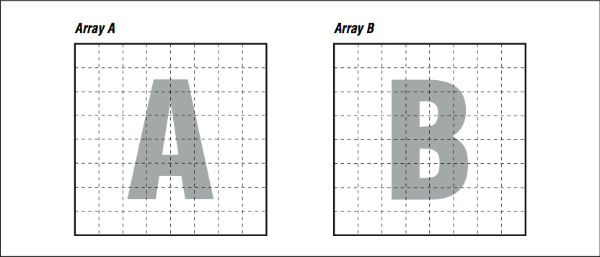
Use your imagination so we can show why this helps. Usually, when we think of a two-dimensional array, we think of a rectangle or a square (see [Figure 1]). Remember, to make programming easier, the compiler provides the illusion that two-dimensional arrays A and B are rectangular plots of memory as in [Figure 1]. Actually, memory is sequential storage. In FORTRAN, a two-dimensional array is constructed in memory by logically lining memory “strips” up against each other, like the pickets of a cedar fence. (It’s the other way around in C: rows are stacked on top of one another.) Array storage starts at the upper left, proceeds down to the bottom, and then starts over at the top of the next column. Stepping through the array with unit stride traces out the shape of a backwards “N,” repeated over and over, moving to the right.

Figure \(\PageIndex{1}\): Arrays A and B

Figure \(\PageIndex{2}\): How array elements are stored

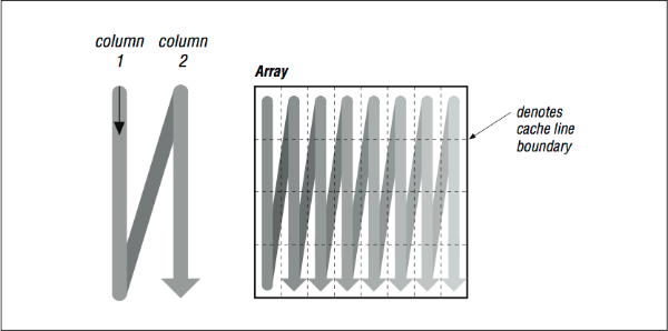
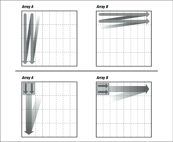
Imagine that the thin horizontal lines of [Figure 2] cut memory storage into pieces the size of individual cache entries. Picture how the loop will traverse them. Because of their index expressions, references to A go from top to bottom (in the backwards “N” shape), consuming every bit of each cache line, but references to B dash off to the right, using one piece of each cache entry and discarding the rest (see [Figure 3], top). This low usage of cache entries will result in a high number of cache misses.

If we could somehow rearrange the loop so that it consumed the arrays in small rectangles, rather than strips, we could conserve some of the cache entries that are being discarded. This is exactly what we accomplished by unrolling both the inner and outer loops, as in the following example. Array A is referenced in several strips side by side, from top to bottom, while B is referenced in several strips side by side, from left to right (see [Figure 3], bottom). This improves cache performance and lowers runtime.

For really big problems, more than cache entries are at stake. On virtual memory machines, memory references have to be translated through a TLB. If you are dealing with large arrays, TLB misses, in addition to cache misses, are going to add to your runtime.

Figure \(\PageIndex{3}\): 2×2 squares

Here’s something that may surprise you. In the code below, we rewrite this loop yet again, this time blocking references at two different levels: in 2×2 squares to save cache entries, and by cutting the original loop in two parts to save TLB entries:

      DO I=1,N,2
        DO J=1,N/2,2
          A(J,I) = A(J,I) + B(I,J)
          A(J+1,I) = A(J+1,I) + B(I+1,J)
          A(J,I+1) = A(J,I+1) + B(I+1,J)
          A(J+1,I+1) = A(J+1,I+1) + B(I+1,J+1)
        ENDDO
      ENDDO
      DO I=1,N,2
        DO J=N/2+1,N,2
          A(J,I) = A(J,I) + B(I,J)
          A(J+1,I) = A(J+1,I) + B(I+1,J)
          A(J,I+1) = A(J,I+1) + B(I+1,J)
          A(J+1,I+1) = A(J+1,I+1) + B(I+1,J+1)
        ENDDO
      ENDDO

You might guess that adding more loops would be the wrong thing to do. But if you work with a reasonably large value of N, say 512, you will see a significant increase in performance. This is because the two arrays A and B are each 256 KB × 8 bytes = 2 MB when N is equal to 512 — larger than can be handled by the TLBs and caches of most processors.

The two boxes in [Figure 4] illustrate how the first few references to A and B look superimposed upon one another in the blocked and unblocked cases. Unblocked references to B zing off through memory, eating through cache and TLB entries. Blocked references are more sparing with the memory system.

Figure \(\PageIndex{4}\): Picture of unblocked versus blocked references

You can take blocking even further for larger problems. This code shows another method that limits the size of the inner loop and visits it repeatedly:

      II = MOD (N,16)
      JJ = MOD (N,4)

      DO I=1,N
        DO J=1,JJ
          A(J,I) = A(J,I) + B(J,I)
        ENDDO
      ENDDO

      DO I=1,II
        DO J=JJ+1,N
            A(J,I) = A(J,I) + B(J,I)
            A(J,I) = A(J,I) + 1.0D0
        ENDDO
      ENDDO

      DO I=II+1,N,16
        DO J=JJ+1,N,4
          DO K=I,I+15
            A(J,K)   = A(J,K)   + B(K,J)
            A(J+1,K) = A(J+1,K) + B(K,J+1)
            A(J+2,K) = A(J+2,K) + B(K,J+2)
            A(J+3,K) = A(J+3,K) + B(K,J+3)
          ENDDO
        ENDDO
      ENDDO

Where the inner I loop used to execute N iterations at a time, the new K loop executes only 16 iterations. This divides and conquers a large memory address space by cutting it into little pieces.

While these blocking techniques begin to have diminishing returns on single-processor systems, on large multiprocessor systems with nonuniform memory access (NUMA), there can be significant benefit in carefully arranging memory accesses to maximize reuse of both cache lines and main memory pages.

Again, the combined unrolling and blocking techniques we just showed you are for loops with mixed stride expressions. They work very well for loop nests like the one we have been looking at. However, if all array references are strided the same way, you will want to try loop unrolling or loop interchange first.

Programs That Require More Memory Than You Have

People occasionally have programs whose memory size requirements are so great that the data can’t fit in memory all at once. At any time, some of the data has to reside outside of main memory on secondary (usually disk) storage. These out-of- core solutions fall into two categories:

• Software-managed, out-of-core solutions
• Virtual memory–managed, out-of-core solutions

With a software-managed approach, the programmer has recognized that the problem is too big and has modified the source code to move sections of the data out to disk for retrieval at a later time. The other method depends on the computer’s memory system handling the secondary storage requirements on its own, some- times at a great cost in runtime.

Software-Managed, Out-of-Core Solutions

Most codes with software-managed, out-of-core solutions have adjustments; you can tell the program how much memory it has to work with, and it takes care of the rest. It is important to make sure the adjustment is set correctly. Code that was tuned for a machine with limited memory could have been ported to another without taking into account the storage available. Perhaps the whole problem will fit easily.

If we are writing an out-of-core solution, the trick is to group memory references together so that they are localized. This usually occurs naturally as a side effect of partitioning, say, a matrix factorization into groups of columns. Blocking references the way we did in the previous section also corrals memory references together so you can treat them as memory “pages.” Knowing when to ship them off to disk entails being closely involved with what the program is doing.

Closing Notes

Loops are the heart of nearly all high performance programs. The first goal with loops is to express them as simply and clearly as possible (i.e., eliminates the clutter). Then, use the profiling and timing tools to figure out which routines and loops are taking the time. Once you find the loops that are using the most time, try to determine if the performance of the loops can be improved.

First try simple modifications to the loops that don’t reduce the clarity of the code. You can also experiment with compiler options that control loop optimizations. Once you’ve exhausted the options of keeping the code looking clean, and if you still need more performance, resort to hand-modifying to the code. Typically the loops that need a little hand-coaxing are loops that are making bad use of the memory architecture on a cache-based system. Hopefully the loops you end up changing are only a few of the overall loops in the program.

However, before going too far optimizing on a single processor machine, take a look at how the program executes on a parallel system. Sometimes the modifications that improve performance on a single-processor system confuses the parallel-processor compiler. The compilers on parallel and vector systems generally have more powerful optimization capabilities, as they must identify areas of your code that will execute well on their specialized hardware. These compilers have been interchanging and unrolling loops automatically for some time now.

Exercises

Exercise \(\PageIndex{1}\)

Why is an unrolling amount of three or four iterations generally sufficient for simple vector loops on a RISC processor? What relationship does the unrolling amount have to floating-point pipeline depths?

Exercise \(\PageIndex{2}\)

On a processor that can execute one floating-point multiply, one floating-point addition/subtraction, and one memory reference per cycle, what’s the best performance you could expect from the following loop?

      DO I = 1,10000
        A(I) = B(I) * C(I) - D(I) * E(I)
      ENDDO

Exercise \(\PageIndex{3}\)

Try unrolling, interchanging, or blocking the loop in subroutine BAZFAZ to increase the performance. What method or combination of methods works best? Look at the assembly language created by the compiler to see what its approach is at the highest level of optimization.

Compile the main routine and BAZFAZ separately; adjust NTIMES so that the untuned run takes about one minute; and use the compiler’s default optimization level.

            PROGRAM MAIN
            IMPLICIT NONE
            INTEGER M,N,I,J
            PARAMETER (N = 512, M = 640, NTIMES = 500)
            DOUBLE PRECISION Q(N,M), R(M,N)
      C
            DO I=1,M
              DO J=1,N
                Q(J,I) = 1.0D0
                R(I,J) = 1.0D0
              ENDDO
            ENDDO
      C
            DO I=1,NTIMES
              CALL BAZFAZ (Q,R,N,M)
            ENDDO
            END

            SUBROUTINE BAZFAZ (Q,R,N,M)
            IMPLICIT NONE
            INTEGER M,N,I,J
            DOUBLE PRECISION Q(N,M), R(N,M)
      C
            DO I=1,N
              DO J=1,M
                R(I,J) = Q(I,J) * R(J,I)
              ENDDO
            ENDDO
      C
            END

Exercise \(\PageIndex{4}\)

Code the matrix multiplication algorithm in the “straightforward” manner and compile it with various optimization levels. See if the compiler performs any type of loop interchange.

Try the same experiment with the following code:

      DO I=1,N
        DO J=1,N
          A(I,J) = A(I,J) + 1.3
        ENDDO
      ENDDO

Do you see a difference in the compiler’s ability to optimize these two loops? If you see a difference, explain it.

Exercise \(\PageIndex{5}\)

Code the matrix multiplication algorithm both the ways shown in this chapter. Execute the program for a range of values for N. Graph the execution time divided by N3 for values of N ranging from 50×50 to 500×500. Explain the performance you see.

---

Footnotes

1. Take a look at the assembly language output to be sure, which may be going a bit overboard. To get an assembly language listing on most machines, compile with the –S flag. On an RS/6000, use the –qlist flag.
2. The compiler reduces the complexity of loop index expressions with a technique called induction variable simplification. See [Section 2.1].
3. It’s also good for improving memory access patterns.
4. When the compiler performs automatic parallel optimization, it prefers to run the outermost loop in parallel to minimize overhead and unroll the innermost loop to make best use of a superscalar or vector processor. For this reason, the compiler needs to have some flexibility in ordering the loops in a loop nest.
5. See [Section 1.1].
6. The Translation Lookaside Buffer (TLB) is a cache of translations from virtual memory addresses to physical memory addresses. For more information, refer back to [Section 1.1].
7. I can’t tell you which is the better way to cast it; it depends on the brand of computer. Some perform better with the loops left as they are, sometimes by more than a factor of two. Others perform better with them interchanged. The difference is in the way the processor handles updates of main memory from cache.