7.1: Infinite Cardinality

uIn the late nineteenth century, the mathematician Georg Cantor was studying the convergence of Fourier series and found some series that he wanted to say converged “most of the time,” even though there were an infinite number of points where they didn’t converge. As a result, Cantor needed a way to compare the size of infinite sets. To get a grip on this, he got the idea of extending the Mapping Rule Theorem 4.5.4 to infinite sets: he regarded two infinite sets as having the “same size” when there was a bijection between them. Likewise, an infinite set \(A\) should be considered “as big as” a set \(B\) when \(A\) surj \(B\). So we could consider \(A\) to be “strictly smaller” than \(B\), which we abbreviate as \(A\) strict \(B\), when \(A\) is not “as big as” \(B\):

Definition \(\PageIndex{1}\)

\[\nonumber A \text{ strict } B \quad \textit{ iff } \quad \text{NOT}(A \text{ surj } B).\]

On finite sets, this strict relation really does mean “strictly smaller.” This follows immediately from the Mapping Rule Theorem 4.5.4.

Corollary 7.1.2. For finite sets \(A, B\),

\[\nonumber A \text{ strict } B  \quad \textit{ iff } \quad |A|<|B|.\]

Proof.

\[\begin{aligned}
A \text { strict } B & \text { iff } \quad \text{NOT}(A \text{ surj } B) & (\text{Def } 7.1.1.) \\
& \text { iff } \quad \text{NOT}(|A| \geq|B|) & (\text{Theorem } 4.5.4. (4.5.1))\\
& \text { iff } \quad|A|<|B|. & \blacksquare
\end{aligned}\]

Cantor got diverted from his study of Fourier series by his effort to develop a theory of infinite sizes based on these ideas. His theory ultimately had profound consequences for the foundations of mathematics and computer science. But Cantor made a lot of enemies in his own time because of his work: the general mathematical community doubted the relevance of what they called “Cantor’s paradise” of unheard-of infinite sizes.

A nice technical feature of Cantor’s idea is that it avoids the need for a definition of what the “size” of an infinite set might be—all it does is compare “sizes.”

Warning: We haven’t, and won’t, define what the “size” of an infinite set is. The definition of infinite “sizes” requires the definition of some infinite sets called ordinals with special well-ordering properties. The theory of ordinals requires getting deeper into technical set theory than we want to go, and we can get by just fine without defining infinite sizes. All we need are the “as big as” and “same size” relations, surj and bij, between sets.

But there’s something else to watch out for: we’ve referred to surj as an “as big as” relation and bij as a “same size” relation on sets. Of course, most of the “as big as” and “same size” properties of surj and bij on finite sets do carry over to infinite sets, but some important ones don’t—as we’re about to show. So you have to be careful: don’t assume that surj has any particular “as big as” property on infinite sets until it’s been proved.

Let’s begin with some familiar properties of the “as big as” and “same size” relations on finite sets that do carry over exactly to infinite sets:

Lemma 7.1.3. For any sets, \(A, B, C\),

1. \(A \text{ surj } B \textit{ iff } B \text{ inj } A\).
2. \(\textit{If } A \text{ surj } B \textit{ and } B \text{ surj } C, \textit{ then } A \text{ surj } C.\)
3. \(\textit{If } A \text{ bij } B \textit{ and } B \text{ bij } C, \textit{ then } A \text{ bij } C.\)
4. \(A \text{ bij } B \textit{ iff } B \text{ bij } A\).

Part 1. follows from the fact that \(R\) has the \([\leq 1 \text{ out}, \geq 1 \text{ in}]\) surjective function property iff \(R^{-1}\) has the \([\geq 1 \text{ out}, \leq 1 \text{ in}]\) total, injective property. Part 2. follows from the fact that compositions of surjections are surjections. Parts 3. and 4. follow from the first two parts because \(R\) is a bijection iff \(R\) and \(R^{-1}\) are surjective functions. We'll leave verification of these facts to Problem 4.22.

Another familiar property of finite sets carries over to infinite sets, but this time some real ingenuity is needed to prove it:

Theorem \(\PageIndex{4}\)

[Schröder-Bernstein] For any sets \(A, B\), \(\textit{if } A \text{ surj } B \textit{ and } B \text{ surj } A, \textit{ then } A \text{ bij } B.\)

That is, the Schröder-Bernstein Theorem says that if \(A\) is at least as big as \(B\) and conversely, \(B\) is at least as big as \(A\), then \(A\) is the same size as \(B\). Phrased this way, you might be tempted to take this theorem for granted, but that would be a mistake. For infinite sets \(A\) and \(B\), the Schröder-Bernstein Theorem is actually pretty technical.

Just because there is a surjective function \(f : A \rightarrow B\)—which need not be a bijection—and a surjective function \(g : B \rightarrow A\)—which also need not be a bijection—it’s not at all clear that there must be a bijection \(e : A \rightarrow B\). The idea is to construct \(e\) from parts of both \(f\) and \(g\). We’ll leave the actual construction to Problem 7.11.

Another familiar set property is that for any two sets, either the first is at least as big as the second, or vice-versa. For finite sets this follows trivially from the Mapping Rule. It’s actually still true for infinite sets, but assuming it was obvious would be mistaken again.

Theorem \(\PageIndex{5}\)

For all sets \(A, B\),

\[\nonumber A \text{ surj } B \text { OR } B \text{ surj } A\]

Theorem 7.1.5 lets us prove that another basic property of finite sets carries over to infinite ones:

Lemma 7.1.6.

\[\label{7.1.1} A \text{ strict } B \text{ AND } B \text{ strict } C\]

implies

\[\nonumber A \text{ strict } C\]

for all sets \(A, B, C\).

Proof. (of Lemma 7.1.6)

Suppose \ref{7.1.1} holds, and assume for the sake of contradiction that \(\text{NOT}(A \text{ strict } C)\), which means that \(A \text{ surj } C\). Now since \(B \text{ strict } C\), Theorem 7.1.5 lets us conclude that \(C \text{ surj } B\). So we have

\[\nonumber A \text{ surj } C \text{ AND } C \text{ surj } B.\]

and Lemma 7.1.3.2 lets us conclude that \(A \text{ surj } B\), contradicting the fact that \(A \text{ strict } B. \quad \blacksquare\)

We’re omitting a proof of Theorem 7.1.5 because proving it involves technical set theory—typically the theory of ordinals again—that we’re not going to get into. But since proving Lemma 7.1.6 is the only use we’ll make of Theorem 7.1.5, we hope you won’t feel cheated not to see a proof.

Infinity is different

A basic property of finite sets that does not carry over to infinite sets is that adding something new makes a set bigger. That is, if \(A\) is a finite set and \(b \notin A\), then \(|A \cup\{b\}|=|A|+1\), and so \(A\) and \(A \cup\{b\}\) are not the same size. But if \(A\) is infinite, then these two sets are the same size!

Lemma 7.1.7. Let \(A\) be a set and \(b \notin A\). Then \(A\) is infinite iff \(A\) bij \(A \cup\{b\}\).

Proof. Since \(A\) is not the same size as \(A \cup\{b\}\) when \(A\) is finite, we only have to show that \(A \cup\{b\}\) is the same size as \(A\) when \(A\) is infinite.

That is, we have to find a bijection between \(A \cup\{b\}\) and \(A\) when \(A\) is infinite. Here’s how: since \(A\) is infinite, it certainly has at least one element; call it \(a_0\). But since \(A\) is infinite, it has at least two elements, and one of them must not equal to \(a_0\); call this new element \(a_1\). But since \(A\) is infinite, it has at least three elements, one of which must not equal both \(a_0\) and \(a_1\); call this new element \(a_2\). Continuing in this way, we conclude that there is an infinite sequence \(a_0, a_1, a_2, \ldots, a_n, \ldots\) of different elements of \(A\). Now it’s easy to define a bijection \(e: A \cup\{b\} \rightarrow A\):

\[\nonumber \begin{array}
e(b) & ::=a_{0}, & \\
e\left(a_{n}\right) & ::=a_{n+1} & \text { for } n \in \mathbb{N}, \\
e(a) & ::=a & \text { for } a \in A-\left\{b, a_{0}, a_{1}, \ldots\right\}. \quad \blacksquare
\end{array}\]

Countable Sets

A set, \(C\), is countable iff its elements can be listed in order, that is, the elements in \(C\) are precisely the elements in the sequence

\[\nonumber c_0, c_1, \ldots, c_n, \ldots\]

Assuming no repeats in the list, saying that \(C\) can be listed in this way is formally the same as saying that the function, \(f : \mathbb{N} \rightarrow C\) defined by the rule that \(f(i) :: c_i\), is a bijection.

Definition \(\PageIndex{8}\)

A set, \(C\), is countably infinite iff \(\mathbb{N} \text{ bij } C\). A set is countable iff it is finite or countably infinite.

We can also make an infinite list using just a finite set of elements if we allow repeats. For example, we can list the elements in the three-element set \({2, 4, 6}\) as

\[\nonumber 2, 4, 6, 6, 6, \ldots\]

This simple observation leads to an alternative characterization of countable sets that does not make separate cases of finite and infinite sets. Namely, a set \(C\) is countable iff there is a list

\[\nonumber c_0, c_1, \ldots, c_n, \ldots\]

of the elements of \(C\), possibly with repeats.

Lemma 7.1.9. A set, \(C\), is countable iff \(\mathbb{N}\) surj \(C\). In fact, a nonempty set \(C\) is countable iff there is a total surjective function \(g : \mathbb{N} \rightarrow C\).

The proof is left to Problem 7.12.

The most fundamental countably infinite set is the set, \(\mathbb{N}\), itself. But the set, \(\mathbb{Z}\), of all integers is also countably infinite, because the integers can be listed in the order:

\[\label{7.1.2} 0, -1, 1, -2, 2, -3, 3, \ldots \]

In this case, there is a simple formula for the \(n\)th element of the list (\ref{7.1.2}). That is, the bijection \(f : \mathbb{N} \rightarrow C\) such that \(f(n)\) is the \(n\)th element of the list can be defined as:

\[\nonumber f(n)::=\left\{\begin{array}{ll}
n / 2 & \text { if } n \text { is even,} \\
-(n+1)/2 & \text { if } n \text { is odd.}
\end{array}\right.\]

There is also a simple way to list all pairs of nonnegative integers, which shows that \((\mathbb{N} \times \mathbb{N})\) is also countably infinite (Problem 7.16). From this, it’s a small step to reach the conclusion that the set, \(\mathbb{Q}^{\geq 0}\), of nonnegative rational numbers is countable. This may be a surprise—after all, the rationals densely fill up the space between integers, and for any two, there’s another in between. So it might seem as though you couldn’t write out all the rationals in a list, but Problem 7.10 illustrates how to do it. More generally, it is easy to show that countable sets are closed under unions and products (Problems 7.1 and 7.16) which implies the countability of a bunch of familiar sets:

Corollary 7.1.10. The following sets are countably infinite:

\[\nonumber \mathbb{Z}^+, \mathbb{Z}, \mathbb{N} \times \mathbb{N}, \mathbb{Q}^+, \mathbb{Z} \times \mathbb{Z}, \mathbb{Q}.\]

A small modification of the proof of Lemma 7.1.7 shows that countably infinite sets are the “smallest” infinite sets, or more precisely that if \(A\) is an infinite set, and \(B\) is countable, then \(A \text{ surj } B\) (see Problem 7.9).

Also, since adding one new element to an infinite set doesn’t change its size, you can add any finite number of elements without changing the size by simply adding one element after another. Something even stronger is true: you can add a countably infinite number of new elements to an infinite set and still wind up with just a set of the same size (Problem 7.13).

By the way, it’s a common mistake to think that, because you can add any finite number of elements to an infinite set and have a bijection with the original set, that you can also throw in infinitely many new elements. In general it isn’t true that just because it’s OK to do something any finite number of times, it also OK to do it an infinite number of times. For example, starting from 3, you can increment by 1 any finite number of times, and the result will be some integer greater than or equal to 3. But if you increment an infinite number of times, you don’t get an integer at all.

Power sets are strictly bigger

Cantor’s astonishing discovery was that not all infinite sets are the same size. In particular, he proved that for any set, \(A\), the power set, pow\((A)\), is “strictly bigger” than \(A\). That is,

Theorem \(\PageIndex{11}\)

[Cantor] For any set, \(A\)

\[\nonumber A \text{ strict pow}(A).\]

Proof. To show that \(A\) is strictly smaller than pow(\(A\)), we have to show that if \(g\) is a function from \(A\) to pow(\(A\)), then \(g\) is not a surjection. To do this, we’ll simply find a subset, \(A_g \subseteq A\) that is not in the range of \(g\). The idea is, for any element \(a \in A\), to look at the set \(g(a) \subseteq A\) and ask whether or not \(a\) happens to be in \(g(a)\). First, define

\[\nonumber A_g ::= \{a \in A \mid a \notin g(a)\}.\]

\(A_g\) is now a well-defined subset of \(A\), which means it is a member of pow\((A)\). But \(A_g\) can’t be in the range of \(g\), because if it were, we would have

\[\nonumber A_g = g(a_0)\]

for some \(a_0 \in A\), so by definition of \(A_g\),

\[\nonumber a \in g(a_0) \text{ iff } a \in A_g \text{ iff } a \notin g(a)\]

for all \(a \in A\). Now letting \(a = a_0\) yields the contradiction

\[\nonumber a_0 \in g(a_0) \text{ iff } a_0 \notin g(a_0).\]

So \(g\) is not a surjection, because there is an element in the power set of \(A\), specifically the set \(A_g\), that is not in the range of \(g\). \(\quad \blacksquare\)

Cantor’s Theorem immediately implies:

Corollary 7.1.12. pow(\(\mathbb{N}\)) is uncountable.

The bijection between subsets of an \(n\)-element set and the length \(n\) bit-strings, \(\{0, 1\}^n\), used to prove Theorem 4.5.5, carries over to a bijection between subsets of a countably infinite set and the infinite bit-strings, \(\{0, 1\}^{\omega}\). That is,

\[\nonumber \text{pow}(\mathbb{N}) \text{ bij } \{0, 1\}^{\omega}.\]

This immediately implies

Corollary 7.1.13. \(\{0, 1\}^{\omega}\) is uncountable.

More Countable and Uncountable Sets

Once we have a few sets we know are countable or uncountable, we can get lots more examples using Lemma 7.1.3. In particular, we can appeal to the following immediate corollary of the Lemma:

Corollary 7.1.14.

(a) If \(U\) is an uncountable set and \(A \text{ surj } U\), then \(A\) is uncountable.

(b) If \(C\) is a countable set and \(C \text{ surj } A\), then \(A\) is countable.

For example, now that we know that the set \(\{0, 1\}^{\omega}\) of infinite bit strings is uncountable, it’s a small step to conclude that

Corollary 7.1.15. The set \(\mathbb{R}\) of real numbers is uncountable.

To prove this, think about the infinite decimal expansion of a real number:

\[\begin{aligned} \sqrt{2} &= 1.4142 \ldots,\\ 5 &= 5.000 \ldots,\\ 1/10 &= 0.1000 \ldots,\\ 1/3 &= 0.333 \ldots,\\ 1/9 &= 0.111 \ldots, \\ 4 \dfrac{1}{99} &= 4.010101 \ldots \end{aligned}\]

Let’s map any real number \(r\) to the infinite bit string \(b(r)\) equal to the sequence of bits in the decimal expansion of \(r\), starting at the decimal point. If the decimal expansion of \(r\) happens to contain a digit other than 0 or 1, leave \(b(r)\) undefined. For example,

\[\begin{aligned} b(5) &= 000 \ldots,\\ b(1/10) &= 1000 \ldots,\\ b(1/9) &= 111 \ldots,\\ b(4\dfrac{1}{99}) &= 010101 \ldots \\ b(\sqrt{2}), b(1/3) &\text{ are undefined.} \end{aligned}\]

Now \(b\) is a function from real numbers to infinite bit strings^.1 It is not a total function, but it clearly is a surjection. This shows that

\[\nonumber \mathbb{R} \text{ surj } \{0, 1\}^{\omega}.\]

and the uncountability of the reals now follows by Corollary 7.1.14.(a).

For another example, let’s prove

Corollary 7.1.16. The set \((\mathbb{Z}^+)^*\) of all finite sequences of positive integers is countable.

To prove this, think about the prime factorization of a nonnegative integer:

\[\begin{aligned} 20 &= 2^2 \cdot 3^0 \cdot 5^1 \cdot 7^0 \cdot 11^0 \cdot 13^0 \ldots , \\ 6615 &= 2^0 \cdot 3^3 \cdot 5^1 \cdot 7^2 \cdot 11^0 \cdot 13^0 \ldots .\end{aligned}\]

Let’s map any nonnegative integer \(n\) to the finite sequence \(e(n)\) of nonzero exponents in its prime factorization. For example,

\[\begin{aligned} e(20) &= (2, 1),\\ e(6615) &= (3, 1, 2), \\ e(5^{13} \cdot 11^9 \cdot 47^{817} \cdot 103^{44}) &= (13, 9, 817, 44), \\ e(1) &= \lambda, & \text{(the empty string)} \\ e(0) &\text{ is undefined.} \end{aligned}\]

Now \(e\) is a function from \(\mathbb{N}\) to \((mathbb{Z}^+)^*\). It is defined on all positive integers, and it clearly is a surjection. This shows that

\[\nonumber \mathbb{N} \text{ surj } (\mathbb{Z}^+)^*.\]

and the countability of the finite strings of positive integers now follows by Corollary 7.1.14.(b).

Larger Infinities

There are lots of different sizes of infinite sets. For example, starting with the infinite set, \(\mathbb{N}\), of nonnegative integers, we can build the infinite sequence of sets

\[\nonumber \mathbb{N} \text{ strict pow}(\mathbb{N}) \text{ strict pow(pow}(\mathbb{N})) \text{ strict pow(pow(pow}(\mathbb{N}))) \text{ strict }\ldots \]

By Cantor’s Theorem 7.1.11, each of these sets is strictly bigger than all the preceding ones. But that’s not all: the union of all the sets in the sequence is strictly bigger than each set in the sequence (see Problem 7.23). In this way you can keep going indefinitely, building “bigger” infinities all the way.

Diagonal Argument

Theorem 7.1.11 and similar proofs are collectively known as “diagonal arguments” because of a more intuitive version of the proof described in terms of on an infinite square array. Namely, suppose there was a bijection between \(\mathbb{N}\) and \(\{0, 1\}^{\omega}\). If such a relation existed, we would be able to display it as a list of the infinite bit strings in some countable order or another. Once we’d found a viable way to organize this list, any given string in \(\{0, 1\}^{\omega}\) would appear in a finite number of steps, just as any integer you can name will show up a finite number of steps from 0. This hypothetical list would look something like the one below, extending to infinity both vertically and horizontally:

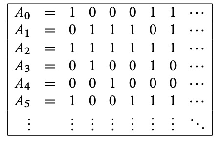
But now we can exhibit a sequence that’s missing from our allegedly complete list of all the sequences. Look at the diagonal in our sample list:

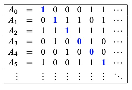
Here is why the diagonal argument has its name: we can form a sequence \(\color{blue}D\) consisting of the bits on the diagonal.

\[\nonumber \color{blue}D \color{black}= \color{blue}1 \quad 1 \quad 1 \quad 0 \quad 0 \quad 1 \ldots, \]

Then, we can form another sequence by switching the \(\color{blue}1\)’s and \(\color{blue}0\)’s along the diagonal. Call this sequence \(\color{red}C\):

\[\nonumber \color{red}C \color{black}= \color{red}0 \quad 0 \quad 0 \quad 1 \quad 1 \quad 0 \ldots. \]

Now if \(n\)th term of \(A_n\) is \(\color{blue}1\) then the \(n\)th term of \(\color{red}C\) is \(\color{red}0\), and vice versa, which guarantees that \(\color{red}C\) differs from \(A_n\). In other words, \(\color{red}C\) has at least one bit different from every sequence on our list. So \(\color{red}C\) is an element of \(\{0, 1\}^{\omega}\) that does not appear in our list—our list can’t be complete!

This diagonal sequence \(\color{red}C\) corresponds to the set \(\{a \in A \mid a \notin g(a)\}\) in the proof of Theorem 7.1.11. Both are defined in terms of a countable subset of the uncountable infinity in a way that excludes them from that subset, thereby proving that no countable subset can be as big as the uncountable set.

 

¹Some rational numbers can be expanded in two ways—as an infinite sequence ending in all 0’s or as an infinite sequence ending in all 9’s. For example,

\begin{aligned} 5 &= 5.000 \ldots = 4.999 \ldots ,\\ \dfrac{1}{10} &= 0.1000 \ldots = 0.0999 \ldots. \end{aligned}

In such cases, define \(b(r)\) to be the sequence that ends with all 0’s.