9.3: Adjacency Matrices

If a graph, \(G\), has \(n\) vertices, \(v_0, v_1, \cdots, v_{n-1}\), a useful way to represent it is with an \(n \times n\) matrix of zeroes and ones called its adjacency matrix, \(A_G\). The ijth entry of the adjacency matrix, \((A_G)_{ij}\), is 1 if there is an edge from vertex \(v_i\) to vertex \(v_j\) and 0 otherwise. That is,

\[\nonumber (A_G)_{ij}::=\left\{\begin{array}{ll}
1 & \text { if } \langle v_i \rightarrow v_j \rangle \in E(G), \\
0 & \text {otherwise.}
\end{array}\right.\]

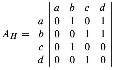
For example, let \(H\) be the 4-node graph shown in Figure 9.1. Its adjacency matrix, \(A_H\), is the \(4 \times 4\) matrix:

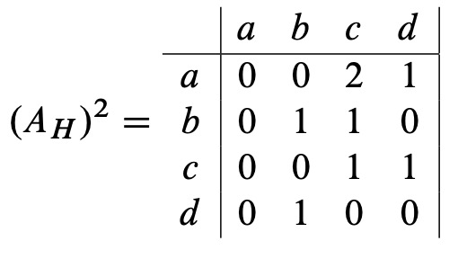
A payoff of this representation is that we can use matrix powers to count numbers of walks between vertices. For example, there are two length two walks between vertices \(a\) and \(c\) in the graph \(H\):

\[\nonumber a \langle a \rightarrow b \rangle b \langle b \rightarrow c \rangle c\]

\[\nonumber a \langle a \rightarrow d \rangle d \langle d \rightarrow c \rangle c\]

and these are the only length two walks from \(a\) to \(c\). Also, there is exactly one length two walk from \(b\) to \(c\) and exactly one length two walk from \(c\) to \(c\) and from \(d\) to \(b\), and these are the only length two walks in \(H\). It turns out we could have read these counts from the entries in the matrix \((A_H)^2\) :

More generally, the matrix \((A_G)^k\) : provides a count of the number of length \(k\) walks between vertices in any digraph, \(G\), as we’ll now explain.

Definition \(\PageIndex{1}\)

The length-\(k\) walk counting matrix for an \(n\)-vertex graph \(G\) is the \(n \times n\) matrix \(C\) such that

\[C_{uv} ::= \text{the number of length-k walks from } u \text{ to } v. \]

Notice that the adjacency matrix \(A_G\) is the length-1 walk counting matrix for \(G\), and that \((A_G)^0\), which by convention is the identity matrix, is the length-0 walk counting matrix.

Theorem \(\PageIndex{2}\)

If \(C\) is the length-\(k\) walk counting matrix for a graph \(G\), and \(D\) is the length-\(m\) walk counting matrix, then \(CD\) is the length \(k + m\) walk counting matrix for \(G\).

According to this theorem, the square \((A_G)^2\) of the adjacency matrix is the length two walk counting matrix for \(G\). Applying the theorem again to \((A_G)^2 A_G\) shows that the length-3 walk counting matrix is \((A_G)^3\). More generally, it follows by induction that

Corollary 9.3.3. The length-k counting matrix of a digraph, \(G\), is \((A_G)^k\), for all \(k \in \mathbb{N}\).

In other words, you can determine the number of length \(k\) walks between any pair of vertices simply by computing the \(k\)th power of the adjacency matrix!

That may seem amazing, but the proof uncovers this simple relationship between matrix multiplication and numbers of walks.

Proof of Theorem 9.3.2. Any length \((k + m)\) walk between vertices \(u\) and \(v\) begins with a length \(k\) walk starting at \(u\) and ending at some vertex, \(w\), followed by a length \(m\) walk starting at \(w\) and ending at \(v\). So the number of length \((k + m)\) walks from \(u\) to \(v\) that go through \(w\) at the \(k\)th step equals the number \(C_{uw}\) of length \(k\) walks from \(u\) to \(w\), times the number \(D_{wv}\) of length \(m\) walks from \(w\) to \(v\). We can get the total number of length \(k + m\) walks from \(u\) to \(v\) by summing, over all possible vertices \(w\), the number of such walks that go through \(w\) at the \(k\)th step. In other words,

\[\label{9.3.2} \# \text{length }(k + m) \text{ walks from } u \text{ to } v = \sum_{u \in V(G)} C_{uw} \cdot D_{wv} \]

But the right hand side of (\ref{9.3.2}) is precisely the definition of \((CD)_{uv}\). Thus, \(CD\) is indeed the length-\((k + m)\) walk counting matrix.

Shortest Paths

The relation between powers of the adjacency matrix and numbers of walks is cool—to us math nerds at least—but a much more important problem is finding shortest paths between pairs of nodes. For example, when you drive home for vacation, you generally want to take the shortest-time route.

One simple way to find the lengths of all the shortest paths in an \(n\)-vertex graph, \(G\), is to compute the successive powers of \(A_G\) one by one up to the \(n - 1\)st, watching for the first power at which each entry becomes positive. That’s because Theorem 9.3.2 implies that the length of the shortest path, if any, between \(u\) and \(v\), that is, the distance from \(u\) to \(v\), will be the smallest value \(k\) for which \((A_G)_{uv}^{k}\) is nonzero, and if there is a shortest path, its length will be \(\leq n - 1\). Refinements of this idea lead to methods that find shortest paths in reasonably efficient ways. The methods apply as well to weighted graphs, where edges are labelled with weights or costs and the objective is to find least weight, cheapest paths. These refinements are typically covered in introductory algorithm courses, and we won’t go into them any further.