9.5: Directed Acyclic Graphs and Scheduling

Some of the prerequisites of MIT computer science subjects are shown in Figure 9.6. An edge going from subject \(s\) to subject \(t\) indicates that \(s\) is listed in the catalogue as a direct prerequisite of \(t\). Of course, before you can take subject \(t\), you have to take not only subject \(s\), but also all the prerequisites of \(s\), and any prerequisites of those prerequisites, and so on. We can state this precisely in terms of the positive walk relation: if \(D\) is the direct prerequisite relation on subjects, then subject \(u\) has to be completed before taking subject \(v\) iff \(u D^+ v\).

Of course it would take forever to graduate if this direct prerequisite graph had a positive length closed walk. We need to forbid such closed walks, which by Lemma 9.2.6 is the same as forbidding cycles. So, the direct prerequisite graph among subjects had better be acyclic:

Definition \(\PageIndex{1}\)

A directed acyclic graph (DAG) is a directed graph with no cycles.

DAGs have particular importance in computer science. They capture key concepts used in analyzing task scheduling and concurrency control. When distributing a program across multiple processors, we’re in trouble if one part of the program needs an output that another part hasn’t generated yet! So let’s examine DAGs and their connection to scheduling in more depth.

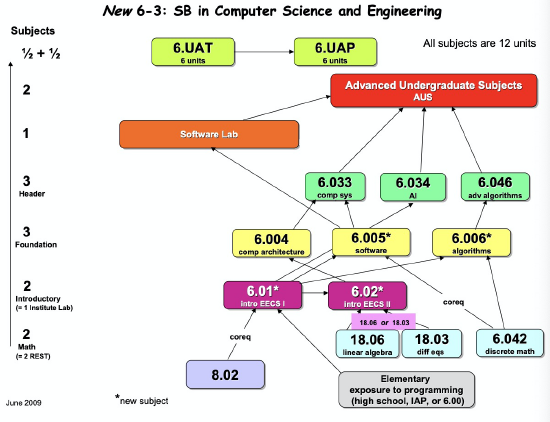
Figure 9.6 Subject prerequisites for MIT Computer Science (6-3) Majors.

Figure 9.7 DAG describing which clothing items have to be put on before others.

Scheduling

In a scheduling problem, there is a set of tasks, along with a set of constraints specifying that starting certain tasks depends on other tasks being completed beforehand. We can map these sets to a digraph, with the tasks as the nodes and the direct prerequisite constraints as the edges.

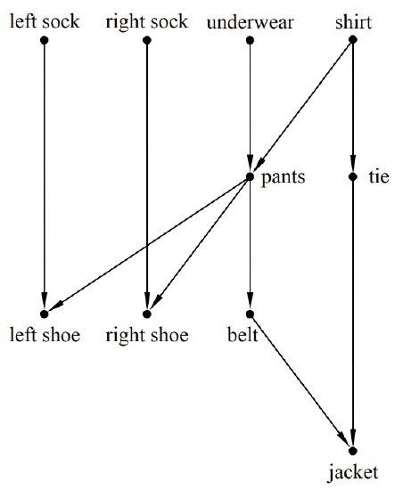
For example, the DAG in Figure 9.7 describes how a man might get dressed for a formal occasion. As we describe above, vertices correspond to garments and the edges specify which garments have to be put on before which others.

When faced with a set of prerequisites like this one, the most basic task is finding an order in which to perform all the tasks, one at a time, while respecting the dependency constraints. Ordering tasks in this way is known as topological sorting.

Definition \(\PageIndex{2}\)

A topological sort of a finite DAG is a list of all the vertices such that each vertex \(v\) appears earlier in the list than every other vertex reachable from \(v\).

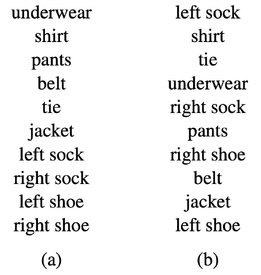
There are many ways to get dressed one item at a time while obeying the constraints of Figure 9.7. We have listed two such topological sorts in Figure 9.8.

Figure 9.8 Two possible topological sorts of the prerequisites described in Figure 9.7

In fact, we can prove that every finite DAG has a topological sort. You can think of this as a mathematical proof that you can indeed get dressed in the morning. Topological sorts for finite DAGs are easy to construct by starting from minimal elements:

Definition \(\PageIndex{3}\)

An vertex \(v\) of a DAG, \(D\), is minimum iff every other vertex is reachable from \(v\).

A vertex \(v\) is minimal iff \(v\) is not reachable from any other vertex.

It can seem peculiar to use the words “minimum” and “minimal” to talk about vertices that start paths. These words come from the perspective that a vertex is “smaller” than any other vertex it connects to. We’ll explore this way of thinking about DAGs in the next section, but for now we’ll use these terms because they are conventional.

One peculiarity of this terminology is that a DAG may have no minimum element but lots of minimal elements. In particular, the clothing example has four minimal elements: leftsock, rightsock, underwear, and shirt.

To build an order for getting dressed, we pick one of these minimal elements— say, shirt. Now there is a new set of minimal elements; the three elements we didn’t chose as step 1 are still minimal, and once we have removed shirt, tie becomes minimal as well. We pick another minimal element, continuing in this way until all elements have been picked. The sequence of elements in the order they were picked will be a topological sort. This is how the topological sorts above were constructed.

So our construction shows:

Theorem \(\PageIndex{4}\)

Every finite DAG has a topological sort.

There are many other ways of constructing topological sorts. For example, instead of starting from the minimal elements at the beginning of paths, we could build a topological sort starting from maximal elements at the end of paths. In fact, we could build a topological sort by picking vertices arbitrarily from a finite DAG and simply inserting them into the list wherever they will fit.⁵

Parallel Task

Scheduling For task dependencies, topological sorting provides a way to execute tasks one after another while respecting those dependencies. But what if we have the ability to execute more than one task at the same time? For example, say tasks are programs, the DAG indicates data dependence, and we have a parallel machine with lots of processors instead of a sequential machine with only one. How should we schedule the tasks? Our goal should be to minimize the total time to complete all the tasks. For simplicity, let’s say all the tasks take the same amount of time and all the processors are identical.

So given a finite set of tasks, how long does it take to do them all in an optimal parallel schedule? We can use walk relations on acyclic graphs to analyze this problem.

In the first unit of time, we should do all minimal items, so we would put on our left sock, our right sock, our underwear, and our shirt.⁶ In the second unit of time, we should put on our pants and our tie. Note that we cannot put on our left or right shoe yet, since we have not yet put on our pants. In the third unit of time, we should put on our left shoe, our right shoe, and our belt. Finally, in the last unit of time, we can put on our jacket. This schedule is illustrated in Figure 9.9.

The total time to do these tasks is 4 units. We cannot do better than 4 units of time because there is a sequence of 4 tasks that must each be done before the next. We have to put on a shirt before pants, pants before a belt, and a belt before a jacket. Such a sequence of items is known as a chain.

Definition \(\PageIndex{5}\)

Two vertices in a DAG are comparable when one of them is reachable from the other. A chain in a DAG is a set of vertices such that any two of them are comparable. A vertex in a chain that is reachable from all other vertices in the chain is called a maximum element of the chain. A finite chain is said to end at its maximum element.

Figure 9.9 A parallel schedule for the tasks-getting-dressed digraph in Figure 9.7. The tasks in \(A_i\) can be performed in step \(i\) for \(1 \leq i \leq 4\). A chain of 4 tasks (the critical path in this example) is shown with bold edges.

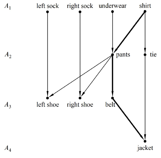
The time it takes to schedule tasks, even with an unlimited number of processors, is at least as large as the number of vertices in any chain. That’s because if we used less time than the size of some chain, then two items from the chain would have to be done at the same step, contradicting the precedence constraints. For this reason, a largest chain is also known as a critical path. For example, Figure 9.9 shows the critical path for the getting-dressed digraph.

In this example, we were able to schedule all the tasks with \(t\) steps, where \(t\) is the size of the largest chain. A nice feature of DAGs is that this is always possible! In other words, for any DAG, there is a legal parallel schedule that runs in \(t\) total steps.

In general, a schedule for performing tasks specifies which tasks to do at successive steps. Every task, \(a\), has to be scheduled at some step, and all the tasks that have to be completed before task \(a\) must be scheduled for an earlier step. Here’s a rigorous definition of schedule.

Definition \(\PageIndex{6}\)

A partition of a set \(A\) is a set of nonempty subsets of \(A\) called the blocks⁷ of the partition, such that every element of \(A\) is in exactly one block.

For example, one possible partition of the set \(\{a, b, c, d, e\}\) into three blocks is

\[\nonumber \{a, c\} \quad \{b, e\} \quad \{d\}.\]

Definition \(\PageIndex{7}\)

A parallel schedule for a DAG, \(D\), is a partition of \(V(D)\) into blocks \(A_0, A_1, \ldots,\) such that when \(j < k\) no vertex in \(A_j\) is reachable from any vertex in \(A_k\). The block \(A_k\) is called the set of elements scheduled at step \(k\), and the time of the schedule is the number of blocks. The maximum number of elements scheduled at any step is called the number of processors required by the schedule.

A largest chain ending at an element \(a\) is called a critical path to \(a\), and the number of elements less than \(a\) in the chain is called the depth of \(a\). So in any possible parallel schedule, there must be at least depth \((a)\) steps before task \(a\) can be started. In particular, the minimal elements are precisely the elements with depth 0.

There is a very simple schedule that completes every task in its minimum number of steps: just use a “greedy” strategy of performing tasks as soon as possible. Schedule all the elements of depth \(k\) at step \(k\). That’s how we found the above schedule for getting dressed.

Theorem \(\PageIndex{8}\)

A minimum time schedule for a finite DAG \(D\) consists of the sets \(A_0, A_1, \ldots,\) where

\[\nonumber A_k ::= \{a \in V(D) \mid \text{depth}(a) = k\}.\]

We’ll leave to Problem 9.19 the proof that the sets \(A_k\) are a parallel schedule according to Definition 9.5.7. We can summarize the story above in this way: with an unlimited number of processors, the parallel time to complete all tasks is simply the size of a critical path:

Corollary 9.5.9. Parallel time = size of critical path.

Things get more complex when the number of processors is bounded; see Problem 9.20 for an example.

Dilworth’s Lemma

Definition \(\PageIndex{10}\)

An antichain in a DAG is a set of vertices such that no two elements in the set are comparable—no walk exists between any two different vertices in the set.

Our conclusions about scheduling also tell us something about antichains.

Corollary 9.5.11. In a DAG, \(D\), if the size of the largest chain is \(t\), then \(V(D)\) can be partitioned into \(t\) antichains.

Proof. Let the antichains be the sets \(A_k ::= \{a \in V(D) \mid \text{depth}(a) = k\}\). It is an easy exercise to verify that each \(A_k\) is an antichain (Problem 9.19). \(\quad \blacksquare\)

Corollary 9.5.11 implies⁸ a famous result about acyclic digraphs:

Lemma 9.5.12 (Dilworth). For all \(t>0\), every DAG with \(n\) vertices must have either a chain of size greater than \(t\) or an antichain of size at least \(n/t\).

Proof. Assume that there is no chain of size greater than \(t\). Let \(\mathcal{l}\) be the size of the largest antichain. If we make a parallel schedule according to the proof of Corollary 9.5.11, we create a number of antichains equal to the size of the largest chain, which is less than or equal \(t\). Each element belongs to exactly one antichain, none of which are larger than \(\mathcal{l}\). So the total number of elements at most \(\mathcal{l}\) times \(t\)—that is, \(\mathcal{l} t \geq n\). Simple division implies that \(\mathcal{l} n/t \quad \blacksquare\).

Corollary 9.5.13. Every DAG with \(n\) vertices has a chain of size greater than \(\sqrt{n}\) or an antichain of size at least \(\sqrt{n}\).

Proof. Set \(t =\sqrt{n}\) in Lemma 9.5.12. \(\quad \blacksquare\)

Example 9.5.14. When the man in our example is getting dressed, \(n = 10\).

Try \(t = 3\). There is a chain of size 4.

Try \(t = 4\). There is no chain of size 5, but there is an antichain of size \(4 \geq 10/4\).

⁵In fact, the DAG doesn’t even need to be finite, but you’ll be relieved to know that we have no need to go into this.

⁶Yes, we know that you can’t actually put on both socks at once, but imagine you are being dressed by a bunch of robot processors and you are in a big hurry. Still not working for you? Ok, forget about the clothes and imagine they are programs with the precedence constraints shown in Figure 9.7.

⁷We think it would be nicer to call them the parts of the partition, but “blocks” is the standard terminology.

⁸Lemma 9.5.12 also follows from a more general result known as Dilworth’s Theorem, which we will not discuss.