10.7: 2-D Array

Last updated
Save as PDF

Page ID: 48362

Eric Lehman, F. Thomson Leighton, & Alberty R. Meyer
Google and Massachusetts Institute of Technology via MIT OpenCourseWare

\( \newcommand{\vecs}[1]{\overset { \scriptstyle \rightharpoonup} {\mathbf{#1}} } \) \( \newcommand{\vecd}[1]{\overset{-\!-\!\rightharpoonup}{\vphantom{a}\smash {#1}}} \)\(\newcommand{\id}{\mathrm{id}}\) \( \newcommand{\Span}{\mathrm{span}}\) \( \newcommand{\kernel}{\mathrm{null}\,}\) \( \newcommand{\range}{\mathrm{range}\,}\) \( \newcommand{\RealPart}{\mathrm{Re}}\) \( \newcommand{\ImaginaryPart}{\mathrm{Im}}\) \( \newcommand{\Argument}{\mathrm{Arg}}\) \( \newcommand{\norm}[1]{\| #1 \|}\) \( \newcommand{\inner}[2]{\langle #1, #2 \rangle}\) \( \newcommand{\Span}{\mathrm{span}}\) \(\newcommand{\id}{\mathrm{id}}\) \( \newcommand{\Span}{\mathrm{span}}\) \( \newcommand{\kernel}{\mathrm{null}\,}\) \( \newcommand{\range}{\mathrm{range}\,}\) \( \newcommand{\RealPart}{\mathrm{Re}}\) \( \newcommand{\ImaginaryPart}{\mathrm{Im}}\) \( \newcommand{\Argument}{\mathrm{Arg}}\) \( \newcommand{\norm}[1]{\| #1 \|}\) \( \newcommand{\inner}[2]{\langle #1, #2 \rangle}\) \( \newcommand{\Span}{\mathrm{span}}\)\(\newcommand{\AA}{\unicode[.8,0]{x212B}}\)

Let’s look at an another communication network. This one is called a 2-dimensional array or grid.

Here there are four inputs and four outputs, so \(N = 4\).

The diameter in this example is 8, which is the number of edges between input 0 and output 3. More generally, the diameter of an array with \(N\) inputs and outputs is \(2N\), which is much worse than the diameter of \(2\log N + 2\) in the complete binary tree. But we get something in exchange: replacing a complete binary tree with an array almost eliminates congestion.

Theorem \(\PageIndex{1}\)

The congestion of an \(N\)-input array is 2.

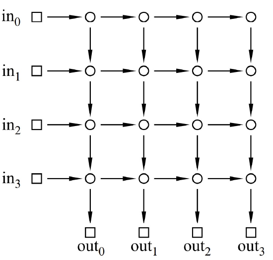
Proof. First, we show that the congestion is at most 2. Let \(\pi\) be any permutation. Define a solution, \(P\), for \(\pi\) to be the set of paths, \(P_i\), where \(P_i\) goes to the right from input \(i\) to column \(\pi(i)\) and then goes down to output \(\pi(i)\). Thus, the switch in row \(i\) and column \(j\) transmits at most two packets: the packet originating at input \(i\) and the packet destined for output \(j\).

Next, we show that the congestion is at least 2. This follows because in any routing problem, \(\pi\), where \(\pi(0) = 0\) and \(\pi(N-1) = N-1\), two packets must pass through the lower left switch. \(\qquad \blacksquare\)

As with the tree, the network latency when minimizing congestion is the same as the diameter. That’s because all the paths between a given input and output are the same length.

Now we can record the characteristics of the 2-D array.

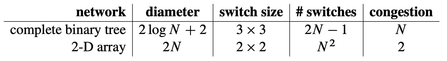
The crucial entry here is the number of switches, which is \(N^2\). This is a major defect of the 2-D array; a network of size \(N = 1000\) would require a million \(2 \times 2\) switches! Still, for applications where \(N\) is small, the simplicity and low congestion of the array make it an attractive choice.