10.9: Beneš Network

In the 1960’s, a researcher at Bell Labs named Václav E. Beneš had a remarkable idea. He obtained a marvelous communication network with congestion 1 by placing two butterflies back-to-back. This amounts to recursively growing Beneš nets by adding both inputs and outputs at each stage. Now we recursively define \(B_n\) to be the switches and connections (without the terminals) of the Beneš net with \(N ::= 2^n\) input and output switches.

The base case, \(B_1\), with 2 input switches and 2 output switches is exactly the same as \(F_1\) in Figure 10.1.

In the constructor step, we construct \(B_{n+1}\) out of two \(B_n\) nets connected to a new set of \(2^{n+1}\) input switches and also a new set of \(2^{n+1}\) output switches. This is illustrated in Figure 10.3.

Figure 10.3 \(B_{n+1}\), the Beneš Net switches with \(2^{n+1}\) inputs and outputs.

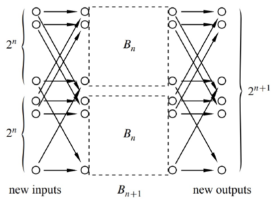
The \(i\)th and \(2^{n+i}\)th new input switches are each connected to the same two switches: the \(i\)th input switches of each of two \(B_n\) components for \(i = 1, ldots, 2^n\), exactly as in the Butterfly net. In addition, the \(i\)th and \(2^{n+i}\)th new output switches are connected to the same two switches, namely, to the \(i\)th output switches of each of two \(B_n\) components.

Now, \(B_{n+1}\) is laid out in columns of height \(2^{n+1}\) by adding two more columns of switches to the columns in \(B_n\). So, the \(B_{n+1}\) switches are arrayed in \(2(n+1)\) columns. The total number of switches is the number of columns times the height of the columns, \(2(n+1)2^{n+1}\).

All paths in \(B_{n+1}\) from an input switch to an output are length \(2(n+1) - 1\), and the diameter of the Beneš net with \(2^{n+1}\) inputs is this length plus two because of the two edges connecting to the terminals.

So Beneš has doubled the number of switches and the diameter, but by doing so he has completely eliminated congestion problems! The proof of this fact relies on a clever induction argument that we’ll come to in a moment. Let’s first see how the Beneš network stacks up:

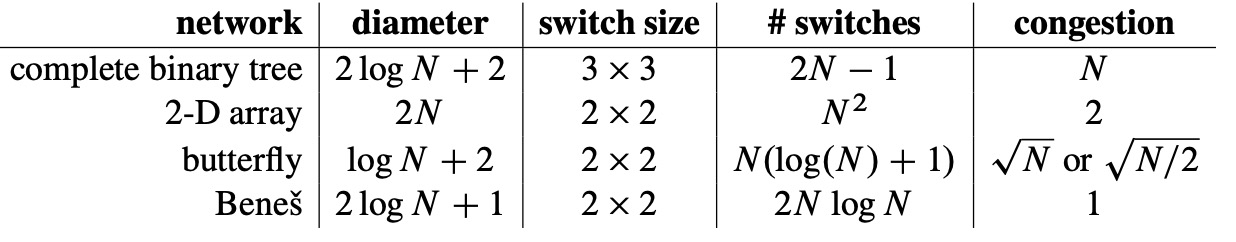
The Beneš network has small size and diameter, and it completely eliminates congestion. The Holy Grail of routing networks is in hand!

Theorem \(\PageIndex{1}\)

The congestion of the \(N\)-input Beneš network is 1.

Proof

By induction on \(n\) where \(N = 2^n\). So the induction hypothesis is

\(P(n) ::= \text{the congestion of }B_n \text{ is } 1.\)

Base case \((n = 1)\): \(B_1 = F_1\) is shown in Figure 10.1. The unique routings in \(F_1\) have congestion 1.

Inductive step: We assume that the congestion of an \(N = 2^n\)-input Beneš network is 1 and prove that the congestion of a \(2N\)-input Beneš network is also 1.

Digression. Time out! Let’s work through an example, develop some intuition, and then complete the proof. In the Beneš network shown in Figure 10.4 with \(N = 8\) inputs and outputs, the two 4-input/output subnetworks are in dashed boxes.

Figure 10.4 Beneš net B3.

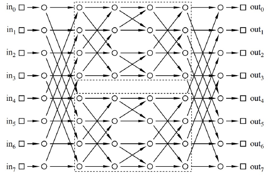
By the inductive assumption, the subnetworks can each route an arbitrary permutation with congestion 1. So if we can guide packets safely through just the first and last levels, then we can rely on induction for the rest! Let’s see how this works in an example. Consider the following permutation routing problem:

\(\begin{aligned} \pi (0) = 1 \qquad \pi (4) = 3 \\ \pi (1) = 5 \qquad \pi (5) = 6 \\ \pi (2) = 4 \qquad \pi (6) = 0 \\ \pi (3) = 7 \qquad \pi (7) = 2 \end{aligned}\)

We can route each packet to its destination through either the upper subnetwork or the lower subnetwork. However, the choice for one packet may constrain the choice for another. For example, we cannot route both packet 0 and packet 4 through the same network, since that would cause two packets to collide at a single switch, resulting in congestion. Rather, one packet must go through the upper network and the other through the lower network. Similarly, packets 1 and 5, 2 and 6, and 3 and 7 must be routed through different networks. Let’s record these constraints in a graph. The vertices are the 8 packets. If two packets must pass through different networks, then there is an edge between them. Thus, our constraint graph looks like this:

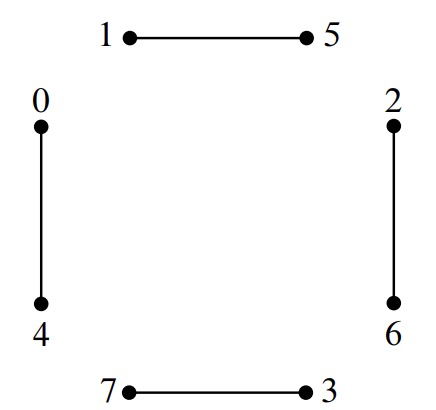
Notice that at most one edge is incident to each vertex.

The output side of the network imposes some further constraints. For example, the packet destined for output 0 (which is packet 6) and the packet destined for output 4 (which is packet 2) cannot both pass through the same network; that would require both packets to arrive from the same switch. Similarly, the packets destined for outputs 1 and 5, 2 and 6, and 3 and 7 must also pass through different switches. We can record these additional constraints in our graph with gray edges:

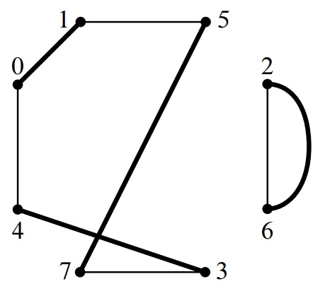
Notice that at most one new edge is incident to each vertex. The two lines drawn between vertices 2 and 6 reflect the two different reasons why these packets must be routed through different networks. However, we intend this to be a simple graph; the two lines still signify a single edge.

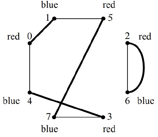
Now here’s the key insight: suppose that we could color each vertex either red or blue so that adjacent vertices are colored differently. Then all constraints are satisfied if we send the red packets through the upper network and the blue packets through the lower network. Such a 2-coloring of the graph corresponds to a solution to the routing problem. The only remaining question is whether the constraint graph is 2-colorable, which is easy to verify:

Lemma 10.9.2. Prove that if the edges of a graph can be grouped into two sets such that every vertex has at most 1 edge from each set incident to it, then the graph is 2-colorable.

Proof. It is not hard to show that a graph is 2-colorable iff every cycle in it has even length (see Theorem 11.9.3). We’ll take this for granted here.

So all we have to do is show that every cycle has even length. Since the two sets of edges may overlap, let’s call an edge that is in both sets a doubled edge.

There are two cases:

Case 1: [The cycle contains a doubled edge.] No other edge can be incident to either of the endpoints of a doubled edge, since that endpoint would then be incident to two edges from the same set. So a cycle traversing a doubled edge has nowhere to go but back and forth along the edge an even number of times.

Case 2: [No edge on the cycle is doubled.] Since each vertex is incident to at most one edge from each set, any path with no doubled edges must traverse successive edges that alternate from one set to the other. In particular, a cycle must traverse a path of alternating edges that begins and ends with edges from different sets. This means the cycle has to be of even length. \(\quad \blacksquare\)

For example, here is a 2-coloring of the constraint graph:

The solution to this graph-coloring problem provides a start on the packet routing problem:

We can complete the routing in the two smaller Beneš networks by induction! Back to the proof. End of Digression.

Let \(\pi\) be an arbitrary permutation of \(\{0, 1, \ldots, N-1\}\). Let \(G\) be the graph whose vertices are packet numbers \(0, 1, \ldots, N-1\) and whose edges come from the union of these two sets:

\[\nonumber \begin{aligned} E_1 &::= \{\langle u - v \rangle \mid |u - v| = N/2\}, \text{ and} \\ E_2 &::= \{\langle u - w \rangle \mid |\pi(u) - \pi(w)| = N/2\}.\end{aligned}\]

Now any vertex, \(u\), is incident to at most two edges: a unique edge \(\langle u - v \rangle \in E_1\) and a unique edge \(\langle u - w \rangle \in E_2\). So according to Lemma 10.9.2, there is a 2- coloring for the vertices of \(G\). Now route packets of one color through the upper subnetwork and packets of the other color through the lower subnetwork. Since for each edge in \(E_1\), one vertex goes to the upper subnetwork and the other to the lower subnetwork, there will not be any conflicts in the first level. Since for each edge in \(E_2\), one vertex comes from the upper subnetwork and the other from the lower subnetwork, there will not be any conflicts in the last level. We can complete the routing within each subnetwork by the induction hypothesis \(P(n). \quad \blacksquare\)