11.5: Bipartite Graphs and Matchings

There were two kinds of vertices in the “Sex in America” graph, males and females, and edges only went between the two kinds. Graphs like this come up so frequently that they have earned a special name: bipartite graphs.

Definition \(\PageIndex{1}\)

A bipartite graph is a graph whose vertices can be partitioned⁴ into two sets, \(L(G)\) and \(R(G)\), such that every edge has one endpoint in \(L(G)\) and the other endpoint in \(R(G)\).

So every bipartite graph looks something like the graph in Figure 11.2.

The Bipartite Matching Problem

The bipartite matching problem is related to the sex-in-America problem that we just studied; only now, the goal is to get everyone happily married. As you might imagine, this is not possible for a variety of reasons, not the least of which is the fact that there are more women in America than men. So, it is simply not possible to marry every woman to a man so that every man is married at most once.

But what about getting a mate for every man so that every woman is married at most once? Is it possible to do this so that each man is paired with a woman that he likes? The answer, of course, depends on the bipartite graph that represents who likes who, but the good news is that it is possible to find natural properties of the who-likes-who graph that completely determine the answer to this question.

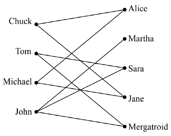
In general, suppose that we have a set of men and an equal-sized or larger set of women, and there is a graph with an edge between a man and a woman if the man likes the woman. In this scenario, the “likes” relationship need not be symmetric, since for the time being, we will only worry about finding a mate for each man that he likes.⁵ (Later, we will consider the “likes” relationship from the female perspective as well.) For example, we might obtain the graph in Figure 11.9.

Figure 11.9 A graph where an edge between a man and woman denotes that the man likes the woman.

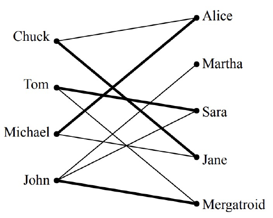
A matching is defined to be an assignment of a woman to each man so that different men are assigned to different women, and a man is always assigned a woman that he likes. For example, one possible matching for the men is shown in Figure 11.10.

Figure 11.10 One possible matching for the men is shown with bold edges. For example, John is matched with Mergatroid.

The Matching Condition

A famous result known as Hall’s Matching Theorem gives necessary and sufficient conditions for the existence of a matching in a bipartite graph. It turns out to be a remarkably useful mathematical tool.

We’ll state and prove Hall’s Theorem using man-likes-woman terminology. Define the set of women liked by a given set of men to consist of all women liked by at least one of those men. For example, the set of women liked by Tom and John in Figure 11.9 consists of Martha, Sara, and Mergatroid. For us to have any chance at all of matching up the men, the following matching condition must hold:

The Matching Condition: every subset of men likes at least as large a set of women.

For example, we cannot find a matching if some set of 4 men like only 3 women. Hall’s Theorem says that this necessary condition is actually sufficient; if the matching condition holds, then a matching exists.

Theorem \(\PageIndex{2}\)

A matching for a set \(M\) of men with a set \(W\) of women can be found if and only if the matching condition holds.

Proof

First, let’s suppose that a matching exists and show that the matching condition holds. For any subset of men, each man likes at least the woman he is matched with and a woman is matched with at most one man. Therefore, every subset of men likes at least as large a set of women. Thus, the matching condition holds.

Next, let’s suppose that the matching condition holds and show that a matching exists. We use strong induction on \(|M|\), the number of men, on the predicate:

\[\nonumber P(m) ::= \text{if the matching condition holds for a set, } M, \text{ of } m \text{ men, then there is a matching for } M.\]

Base case (\(|M| = 1\)): If \(|M| = 1\), then the matching condition implies that the lone man likes at least one woman, and so a matching exists.

Inductive Step: Suppose that \(|M| = m + 1 \geq 2\). To find a matching for \(M\), there are two cases.

Case 1: Every nonempty subset of at most \(m\) men likes a strictly larger set of women. In this case, we have some latitude: we pair an arbitrary man with a woman he likes and send them both away. This leaves \(m\) men and one fewer women, and the matching condition will still hold. So the induction hypothesis \(P(m)\) implies we can match the remaining \(m\) men.

Case 2: Some nonempty subset, \(X\), of at most \(m\) men likes an equal-size set, \(Y\), of women. The matching condition must hold within \(X\), so the strong induction hypothesis implies we can match the men in \(X\) with the women in \(Y\). This leaves the problem of matching the set \(M - X\) of men to the set \(W - Y\) of women.

But the problem of matching \(M - X\) against \(W - Y\) also satisfies the Matching condition, because any subset of men in \(M - X\) who liked fewer women in \(W - Y\) would imply there was a set of men who liked fewer women in the whole set \(W\). Namely, if a subset \(M_0 \subseteq M - X\) liked only a strictly smaller subset of women \(W_0 \subseteq W - Y\), then the set \(M_0 \cup X\) of men would like only women in the strictly smaller set \(W_0 \cup Y\). So again the strong induction hypothesis implies we can match the men in \(M - X\) with the women in \(W - Y\), which completes a matching for \(M\).

So in both cases, there is a matching for the men, which completes the proof of the Inductive step. The theorem follows by induction. \(\quad \blacksquare\)

The proof of Theorem 11.5.2 gives an algorithm for finding a matching in a bipartite graph, albeit not a very efficient one. However, efficient algorithms for finding a matching in a bipartite graph do exist. Thus, if a problem can be reduced to finding a matching, the problem is essentially solved from a computational perspective.

A Formal Statement

Let’s restate Theorem 11.5.2 in abstract terms so that you’ll not always be condemned to saying, “Now this group of men likes at least as many women. . . ”

Definition \(\PageIndex{3}\)

A matching in a graph \(G\) is a set \(M\) of edges of \(G\) such that no vertex is an endpoint of more than one edge in \(M\). A matching is said to cover a set, \(S\), of vertices iff each vertex in \(S\) is an endpoint of an edge of the matching. A matching is said to be perfect if it covers \(V(G)\). In any graph, \(G\), the set \(N(S)\) of neighbors of some set \(S\) of vertices is the image of \(S\) under the edge-relation, that is,

\[\nonumber N(S) ::= \{r \mid \langle s - r \rangle \in E(G) \text{ for some } s \in S\}.\]

\(S\) is called a bottleneck if

\[\nonumber |S| > |N(S)|.\]

Theorem \(\PageIndex{4}\)

(Hall’s Theorem). Let \(G\) be a bipartite graph. There is a matching in \(G\) that covers \(L(G)\) iff no subset of \(L(G)\) is a bottleneck.

An Easy Matching Condition

The bipartite matching condition requires that every subset of men has a certain property. In general, verifying that every subset has some property, even if it’s easy to check any particular subset for the property, quickly becomes overwhelming because the number of subsets of even relatively small sets is enormous—over a billion subsets for a set of size 30. However, there is a simple property of vertex degrees in a bipartite graph that guarantees the existence of a matching. Call a bipartite graph degree-constrained if vertex degrees on the left are at least as large as those on the right. More precisely,

Definition \(\PageIndex{5}\)

A bipartite graph \(G\) is degree-constrained when \(\text{deg}(l) \geq \text{deg}(r)\) for every \(l \in L(G)\) and \(r \in R(G)\).

For example, the graph in Figure 11.9 is degree-constrained since every node on the left is adjacent to at least two nodes on the right while every node on the right is adjacent to at most two nodes on the left.

Theorem \(\PageIndex{6}\)

If \(G\) is a degree-constrained bipartite graph, then there is a matching that covers \(L(G)\).

Proof

We will show that \(G\) satisfies Hall’s condition, namely, if \(S\) is an arbitrary subset of \(L(G)\), then

\[\label{11.5.1} |N(S)| \geq |S|.\]

Since \(G\) is degree-constrained, there is a \(d>0\) such that \(\text{deg}(l) \geq d \geq \text{deg}(r)\) for every \(l \in L\) and \(r \in R\). Since every edge with an endpoint in \(S\) has its other endpoint in \(N(S)\) by definition, and every node in \(N(S)\) is incident to at most \(d\) edges, we know that

\[\nonumber d |N(S)| \geq \text{ #edges with an endpoint in } S.\]

Also, since every node in \(S\) is the endpoint of at least \(d\) edges,

\[\nonumber \text{ #edges incident to a vertex in } S \geq d|S|.\]

It follows that \(d |N(S)| \geq d|S|\). Cancelling \(d\) completes the derivation of equation (\(\ref{11.5.1}\)).

Regular graphs are a large class of degree-constrained graphs that often arise in practice. Hence, we can use Theorem 11.5.6 to prove that every regular bipartite graph has a perfect matching. This turns out to be a surprisingly useful result in computer science.

Definition \(\PageIndex{7}\)

A graph is said to be regular if every node has the same degree.

Theorem \(\PageIndex{8}\)

Every regular bipartite graph has a perfect matching.

Proof

Let \(G\) be a regular bipartite graph. Since regular graphs are degree-constrained, we know by Theorem 11.5.6 that there must be a matching in \(G\) that covers \(L(G)\). Such a matching is only possible when \(|L(G)| \leq |R(G)|\). But \(G\) is also degreeconstrained if the roles of \(L(G)\) and \(R(G)\) are switched, which implies that \(|R(G)| \leq |L(G)|\) also. That is, \(L(G)\) and \(R(G)\) are the same size, and any matching covering \(L(G)\) will also cover \(R(G)\). So every node in \(G\) is an endpoint of an edge in the matching, and thus \(G\) has a perfect matching. \(\quad \blacksquare\)

⁴Partitioning a set means cutting it up into nonempty pieces. In this case, it means that \(L(G)\) and \(R(G)\) are nonempty, \(L(G) \cup R(G) = V(G)\), and \(L(G) \cap R(G) = \emptyset\).

⁵By the way, we do not mean to imply that marriage should or should not be heterosexual. Nor do we mean to imply that men should get their choice instead of women. It’s just that there are fewer men than women in America, making it impossible to match up all the women with different men. So please don’t take offense.