11.7: Coloring

In Section 11.2, we used edges to indicate an affinity between a pair of nodes. But there are lots of situations in which edges will correspond to conflicts between nodes. Exam scheduling is a typical example.

Exam Scheduling Problem

Each term, the MIT Schedules Office must assign a time slot for each final exam. This is not easy, because some students are taking several classes with finals, and (even at MIT) a student can take only one test during a particular time slot. The Schedules Office wants to avoid all conflicts. Of course, you can make such a schedule by having every exam in a different slot, but then you would need hundreds of slots for the hundreds of courses, and the exam period would run all year! So, the Schedules Office would also like to keep exam period short.

The Schedules Office’s problem is easy to describe as a graph. There will be a vertex for each course with a final exam, and two vertices will be adjacent exactly when some student is taking both courses. For example, suppose we need to schedule exams for 6.041, 6.042, 6.002, 6.003 and 6.170. The scheduling graph might appear as in Figure 11.12.

Figure 11.12 A scheduling graph for five exams. Exams connected by an edge cannot be given at the same time.

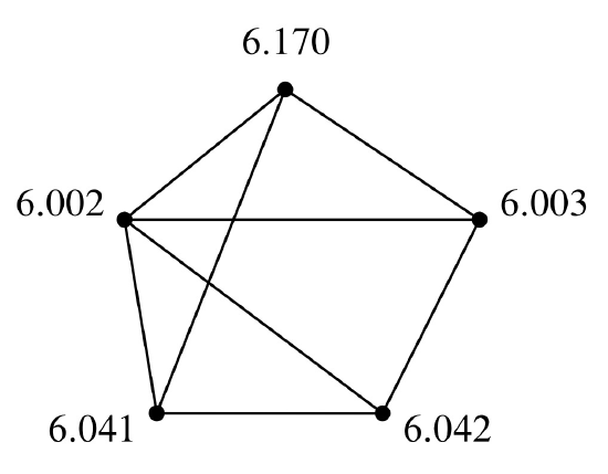
6.002 and 6.042 cannot have an exam at the same time since there are students in both courses, so there is an edge between their nodes. On the other hand, 6.042 and 6.170 can have an exam at the same time if they’re taught at the same time (which they sometimes are), since no student can be enrolled in both (that is, no student should be enrolled in both when they have a timing conflict).

We next identify each time slot with a color. For example, Monday morning is red, Monday afternoon is blue, Tuesday morning is green, etc. Assigning an exam to a time slot is then equivalent to coloring the corresponding vertex. The main constraint is that adjacent vertices must get different colors—otherwise, some student has two exams at the same time. Furthermore, in order to keep the exam period short, we should try to color all the vertices using as few different colors as possible. As shown in Figure 11.13, three colors suffice for our example.

Figure 11.13 A 3-coloring of the exam graph from Figure 11.12.

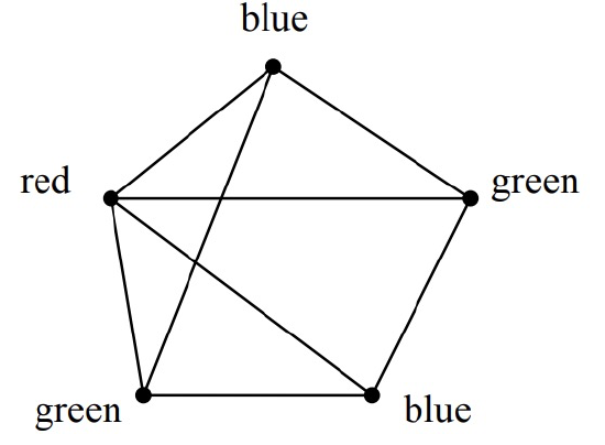
The coloring in Figure 11.13 corresponds to giving one final on Monday morning (red), two Monday afternoon (blue), and two Tuesday morning (green). Can we use fewer than three colors? No! We can’t use only two colors since there is a triangle in the graph, and three vertices in a triangle must all have different colors.

This is an example of a graph coloring problem: given a graph \(G\), assign colors to each node such that adjacent nodes have different colors. A color assignment with this property is called a valid coloring of the graph—a “coloring,” for short. A graph \(G\) is \(k\)-colorable if it has a coloring that uses at most \(k\) colors.

Definition \(\PageIndex{1}\)

The minimum value of \(k\) for which a graph, \(G\), has a valid coloring is called its chromatic number, \(\chi (G)\).

So \(G\) is \(k\)-colorable iff \(\chi (G) \leq k\).

In general, trying to figure out if you can color a graph with a fixed number of colors can take a long time. It’s a classic example of a problem for which no fast algorithms are known. In fact, it is easy to check if a coloring works, but it seems really hard to find it. (If you figure out how, then you can get a $1 million Clay prize.)

Some Coloring Bounds

There are some simple properties of graphs that give useful bounds on colorability. The simplest property is being a cycle: an even-length closed cycle is 2-colorable. Cycles in simple graphs by convention have positive length and so are not 1- colorable. So

\[\nonumber \chi (C_{even}) = 2.\]

On the other hand, an odd-length cycle requires 3 colors, that is,

\[\label{11.7.1} \chi (C_{odd}) = 3.\]

You should take a moment to think about why this equality holds.

Another simple example is a complete graph \(K_n\):

\[\nonumber \chi (K_n) = n\]

since no two vertices can have the same color.

Being bipartite is another property closely related to colorability. If a graph is bipartite, then you can color it with 2 colors using one color for the nodes on the “left” and a second color for the nodes on the “right.” Conversely, graphs with chromatic number 2 are all bipartite with all the vertices of one color on the “left” and those with the other color on the right. Since only graphs with no edges—the empty graphs—have chromatic number 1, we have:

Lemma 11.7.2. A graph, \(G\), with at least one edge is bipartite iff \(\chi (G) = 2\).

The chromatic number of a graph can also be shown to be small if the vertex degrees of the graph are small. In particular, if we have an upper bound on the degrees of all the vertices in a graph, then we can easily find a coloring with only one more color than the degree bound.

Theorem \(\PageIndex{4}\)

A graph with maximum degree at most \(k\) is \(k + 1\)-colorable.

Since \(k\) is the only nonnegative integer valued variable mentioned in the theorem, you might be tempted to try to prove this theorem using induction on \(k\). Unfortunately, this approach leads to disaster—we don’t know of any reasonable way to do this and expect it would ruin your week if you tried it on a problem set. When you encounter such a disaster using induction on graphs, it is usually best to change what you are inducting on. In graphs, typical good choices for the induction parameter are \(n\), the number of nodes, or \(e\), the number of edges.

Proof

We use induction on the number of vertices in the graph, which we denote by \(n\). Let \(P(n)\) be the proposition that an \(n\)-vertex graph with maximum degree at most \(k\) is \(k+1\)-colorable.

Base case (\(n = 1\)): A 1-vertex graph has maximum degree 0 and is 1-colorable, so \(P(1)\) is true.

Inductive step: Now assume that \(P(n)\) is true, and let \(G\) be an \((n+1)\)-vertex graph with maximum degree at most \(k\). Remove a vertex \(v\) (and all edges incident to it), leaving an \(n\)-vertex subgraph, \(H\). The maximum degree of \(H\) is at most \(k\), and so \(H\) is \((k+1)\)-colorable by our assumption \(P(n)\). Now add back vertex \(v\). We can assign \(v\) a color (from the set of \((k+1)\) colors) that is different from all its adjacent vertices, since there are at most \(k\) vertices adjacent to \(v\) and so at least one of the \((k+1)\) colors is still available. Therefore, \(G\) is \((k+1)\)-colorable. This completes the inductive step, and the theorem follows by induction. \(\quad \blacksquare\)

Sometimes \(k + 1\) colors is the best you can do. For example, \(\chi(K_n) = n\)and every node in \(K_n\) has degree \(k = n - 1\) and so this is an example where Theorem 11.7.3 gives the best possible bound. By a similar argument, we can show that Theorem 11.7.3 gives the best possible bound for any graph with degree bounded by \(k\) that has \(K_{k+1}\) as a subgraph.

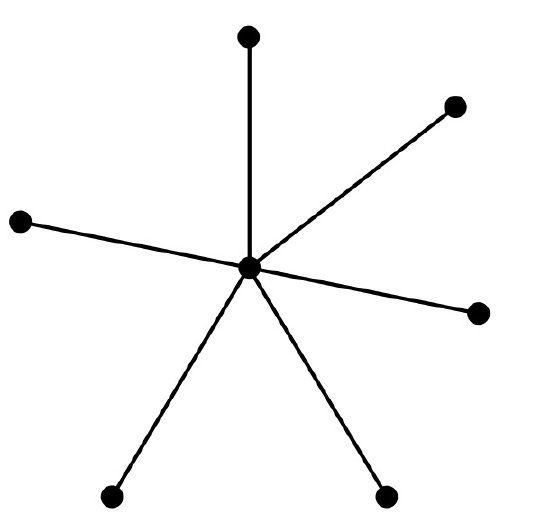
But sometimes \(k + 1\) colors is far from the best that you can do. For example, the \(n\)-node star graph shown in Figure 11.14 has maximum degree \(n - 1\) but can be colored using just 2 colors.

Figure 11.14 A 7-node star graph.

Why coloring?

One reason coloring problems frequently arise in practice is because scheduling conflicts are so common. For example, at Akamai, a new version of software is deployed over each of 65,000 servers every few days. The updates cannot be done at the same time since the servers need to be taken down in order to deploy the software. Also, the servers cannot be handled one at a time, since it would take forever to update them all (each one takes about an hour). Moreover, certain pairs of servers cannot be taken down at the same time since they have common critical functions. This problem was eventually solved by making a 65,000-node conflict graph and coloring it with 8 colors—so only 8 waves of install are needed!

Another example comes from the need to assign frequencies to radio stations. If two stations have an overlap in their broadcast area, they can’t be given the same frequency. Frequencies are precious and expensive, so you want to minimize the number handed out. This amounts to finding the minimum coloring for a graph whose vertices are the stations and whose edges connect stations with overlapping areas.

Coloring also comes up in allocating registers for program variables. While a variable is in use, its value needs to be saved in a register. Registers can be reused for different variables but two variables need different registers if they are referenced during overlapping intervals of program execution. So register allocation is the coloring problem for a graph whose vertices are the variables: vertices are adjacent if their intervals overlap, and the colors are registers. Once again, the goal is to minimize the number of colors needed to color the graph.

Finally, there’s the famous map coloring problem stated in Proposition 1.1.6. The question is how many colors are needed to color a map so that adjacent territories get different colors? This is the same as the number of colors needed to color a graph that can be drawn in the plane without edges crossing. A proof that four colors are enough for planar graphs was acclaimed when it was discovered about thirty years ago. Implicit in that proof was a 4-coloring procedure that takes time proportional to the number of vertices in the graph (countries in the map).

Surprisingly, it’s another of those million dollar prize questions to find an efficient procedure to tell if a planar graph really needs four colors, or if three will actually do the job. A proof that testing 3-colorability of graphs is as hard as the million dollar SAT problem is given in Problem 11.39; this turns out to be true even for planar graphs. (It is easy to tell if a graph is 2-colorable, as explained in Section 11.9.2.) In Chapter 12, we’ll develop enough planar graph theory to present an easy proof that all planar graphs are 5-colorable.