16.2: The Four Step Method

Every probability problem involves some sort of randomized experiment, process, or game. And each such problem involves two distinct challenges:

1. How do we model the situation mathematically?
2. How do we solve the resulting mathematical problem?

In this section, we introduce a four step approach to questions of the form, “What is the probability that. . . ?” In this approach, we build a probabilistic model step by step, formalizing the original question in terms of that model. Remarkably, this structured approach provides simple solutions to many famously confusing problems. For example, as you’ll see, the four step method cuts through the confusion surrounding the Monty Hall problem like a Ginsu knife.

Step 1: Find the Sample Space

Our first objective is to identify all the possible outcomes of the experiment. A typical experiment involves several randomly-determined quantities. For example, the Monty Hall game involves three such quantities:

1. The door concealing the car.
2. The door initially chosen by the player.
3. The door that the host opens to reveal a goat.

Every possible combination of these randomly-determined quantities is called an outcome. The set of all possible outcomes is called the sample space for the experiment.

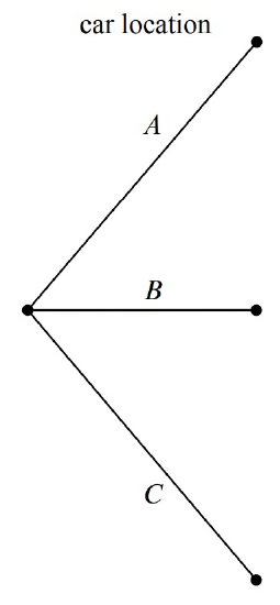
A tree diagram is a graphical tool that can help us work through the four step approach when the number of outcomes is not too large or the problem is nicely structured. In particular, we can use a tree diagram to help understand the sample space of an experiment. The first randomly-determined quantity in our experiment is the door concealing the prize. We represent this as a tree with three branches, as shown in Figure 16.1. In this diagram, the doors are called A, B, and C instead of \(1, 2,\) and \(3\), because we’ll be adding a lot of other numbers to the picture later.

Figure 16.1 The first level in a tree diagram for the Monty Hall Problem. The branches correspond to the door behind which the car is located.

For each possible location of the prize, the player could initially choose any of the three doors. We represent this in a second layer added to the tree. Then a third layer represents the possibilities of the final step when the host opens a door to reveal a goat, as shown in Figure 16.2

Figure 16.2 The full tree diagram for the Monty Hall Problem. The second level indicates the door initially chosen by the player. The third level indicates the door revealed by Monty Hall.

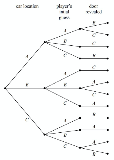
Notice that the third layer reflects the fact that the host has either one choice or two, depending on the position of the car and the door initially selected by the player. For example, if the prize is behind door A and the player picks door B, then the host must open door C. However, if the prize is behind door A and the player picks door A, then the host could open either door B or door C.

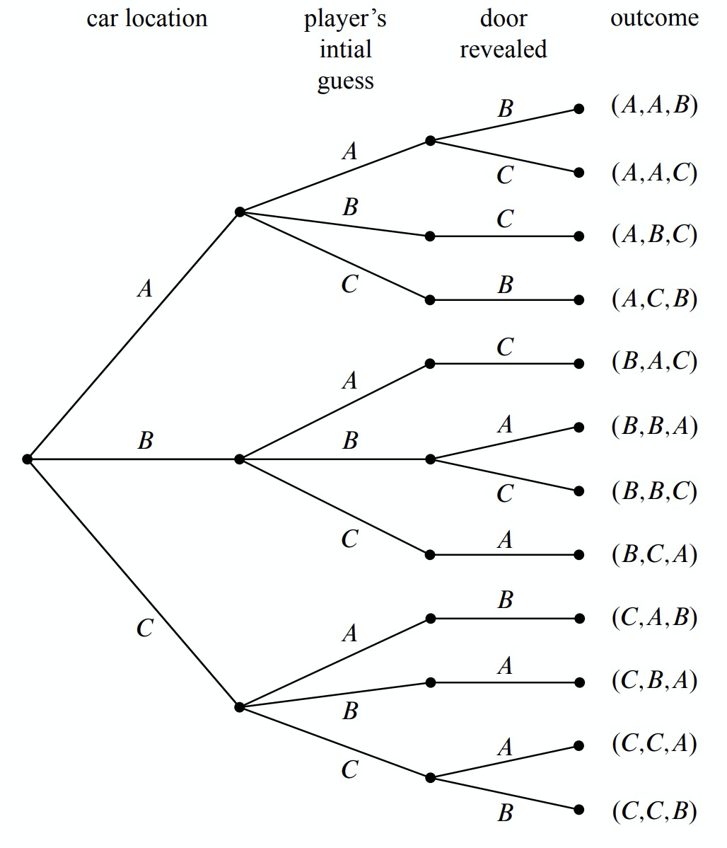
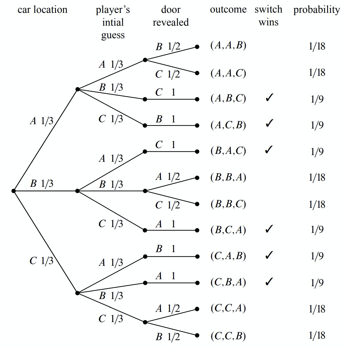
Now let’s relate this picture to the terms we introduced earlier: the leaves of the tree represent outcomes of the experiment, and the set of all leaves represents the sample space. Thus, for this experiment, the sample space consists of 12 outcomes. For reference, we’ve labeled each outcome in Figure 16.3 with a triple of doors indicating:

(door concealing prize, door initially chosen, door opened to reveal a goat).

Figure 16.3 The tree diagram for the Monty Hall Problem with the outcomes labeled for each path from root to leaf. For example, outcome \((A, A, B)\) corresponds to the car being behind door \(A\), the player initially choosing door \(A\), and Monty Hall revealing the goat behind door \(B\).

In these terms, the sample space is the set

\[\nonumber S = \left\{\begin{array}{l}
(A, A, B), (A, A, C), (A, B, C), (A, C, B), (B, A, C), (B, B, A), \\
(B, B, C), (B, C, A), (C, A, B), (C, B, A), (C, C, A), (C, C, B) \\
\end{array}\right\}\]

The tree diagram has a broader interpretation as well: we can regard the whole experiment as following a path from the root to a leaf, where the branch taken at each stage is “randomly” determined. Keep this interpretation in mind; we’ll use it again later.

Step 2: Define Events of Interest

Our objective is to answer questions of the form “What is the probability that . . . ?”, where, for example, the missing phrase might be “the player wins by switching,” “the player initially picked the door concealing the prize,” or “the prize is behind door C.”

A set of outcomes is called an event. Each of the preceding phrases characterizes an event. For example, the event [prize is behind door \(C\)] refers to the set:

\[\nonumber \{(C, A, B), (C, B, A), (C, C, A), (C, C, B)\},\]

and the event [prize is behind the door first picked by the player] is:

\[\nonumber \{(A, A, B), (A, A, C), (B, B, A), (B, B, C), (C, C, A), (C, C, B)\}.\]

Here we’re using square brackets around a property of outcomes as a notation for the event whose outcomes are the ones that satisfy the property.

What we’re really after is the event [player wins by switching]:

\[\label{16.2.1} \{(A, B, C), (A, C, B), (B, A, C), (B, C, A), (C, A, B), (C, B, A)\}.\]

The outcomes in this event are marked with checks in Figure 16.4.

Figure 16.4 The tree diagram for the Monty Hall Problem, where the outcomes where the player wins by switching are denoted with a check mark.

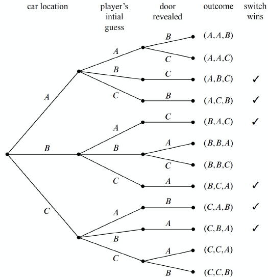
Notice that exactly half of the outcomes are checked, meaning that the player wins by switching in half of all outcomes. You might be tempted to conclude that a player who switches wins with probability \(1/2\). This is wrong. The reason is that these outcomes are not all equally likely, as we’ll see shortly.

Step 3: Determine Outcome Probabilities

So far we’ve enumerated all the possible outcomes of the experiment. Now we must start assessing the likelihood of those outcomes. In particular, the goal of this step is to assign each outcome a probability, indicating the fraction of the time this outcome is expected to occur. The sum of all the outcome probabilities must equal one, reflecting the fact that there always must be an outcome.

Ultimately, outcome probabilities are determined by the phenomenon we’re modeling and thus are not quantities that we can derive mathematically. However, mathematics can help us compute the probability of every outcome based on fewer and more elementary modeling decisions. In particular, we’ll break the task of determining outcome probabilities into two stages.

Step 3a: Assign Edge Probabilities

First, we record a probability on each edge of the tree diagram. These edgeprobabilities are determined by the assumptions we made at the outset: that the prize is equally likely to be behind each door, that the player is equally likely to pick each door, and that the host is equally likely to reveal each goat, if he has a choice. Notice that when the host has no choice regarding which door to open, the single branch is assigned probability 1. For example, see Figure 16.5.

Figure 16.5 The tree diagram for the Monty Hall Problem where edge weights denote the probability of that branch being taken given that we are at the parent of that branch. For example, if the car is behind door \(A\), then there is a 1/3 chance that the player’s initial selection is door \(B\). The rightmost column shows the outcome probabilities for the Monty Hall Problem. Each outcome probability is simply the product of the probabilities on the path from the root to the outcome leaf.

Step 3b: Compute Outcome Probabilities

Our next job is to convert edge probabilities into outcome probabilities. This is a purely mechanical process:

calculate the probability of an outcome by multiplying the edge-probabilities on the path from the root to that outcome.

For example, the probability of the topmost outcome in Figure 16.5, \((A, A, B)\), is

\[\label{16.2.2} \frac{1}{3} \cdot \frac{1}{3} \cdot \frac{1}{2} = \frac{1}{18}.\]

We’ll examine the official justification for this rule in Section 17.4, but here’s an easy, intuitive justification: as the steps in an experiment progress randomly along a path from the root of the tree to a leaf, the probabilities on the edges indicate how likely the path is to proceed along each branch. For example, a path starting at the root in our example is equally likely to go down each of the three top-level branches.

How likely is such a path to arrive at the topmost outcome, \((A, A, B)\)? Well, there is a 1-in-3 chance that a path would follow the \(A\)-branch at the top level, a 1-in-3 chance it would continue along the \(A\)-branch at the second level, and 1-in-2 chance it would follow the \(B\)-branch at the third level. Thus, there is half of a one third of a one third chance, of arriving at the \((A, A, B)\) leaf. That is, the chance is \(1/3 \cdot 1/3 \cdot 1/2 = 1/18\)—the same product (in reverse order) we arrived at in (\ref{16.2.2}).

We have illustrated all of the outcome probabilities in Figure 16.5.

Specifying the probability of each outcome amounts to defining a function that maps each outcome to a probability. This function is usually called \(\text{Pr}[-]\). In these terms, we’ve just determined that:

\[\begin{aligned} \text{Pr}[(A, A, B)] &= \frac{1}{18}, \\ \text{Pr}[(A, A, C)] &= \frac{1}{18}, \\ \text{Pr}[(A, B, C)] &= \frac{1}{9}, \\ &\text{etc}. \end{aligned}\]

Step 4: Compute Event Probabilities

We now have a probability for each outcome, but we want to determine the probability of an event. The probability of an event \(E\) is denoted by \(\text{Pr}[E]\), and it is the sum of the probabilities of the outcomes in \(E\). For example, the probability of the [switching wins] event (\ref{16.2.1}) is

\[\begin{aligned} &\text{Pr [switching wins]} \\ &= \text{Pr}[(A, B, C)] + \text{Pr}[(A, C, B)] + \text{Pr}[(B, A, C)] + \text{Pr}[(B, C, A)] + \text{Pr}[(C, A, B)] + \text{Pr}[(C, B, A)] \\ &= \frac{1}{9} + \frac{1}{9} + \frac{1}{9} + \frac{1}{9} + \frac{1}{9} + \frac{1}{9} \\ &= \frac{2}{3}. \end{aligned}\]

It seems Marilyn’s answer is correct! A player who switches doors wins the car with probability \(2/3\). In contrast, a player who stays with his or her original door wins with probability \(1/3\), since staying wins if and only if switching loses.

We’re done with the problem! We didn’t need any appeals to intuition or ingenious analogies. In fact, no mathematics more difficult than adding and multiplying fractions was required. The only hard part was resisting the temptation to leap to an “intuitively obvious” answer.

Alternative Interpretation of the Monty Hall Problem

Was Marilyn really right? Our analysis indicates that she was. But a more accurate conclusion is that her answer is correct provided we accept her interpretation of the question. There is an equally plausible interpretation in which Marilyn’s answer is wrong. Notice that Craig Whitaker’s original letter does not say that the host is required to reveal a goat and offer the player the option to switch, merely that he did these things. In fact, on the Let’s Make a Deal show, Monty Hall sometimes simply opened the door that the contestant picked initially. Therefore, if he wanted to, Monty could give the option of switching only to contestants who picked the correct door initially. In this case, switching never works!