18.3: Distribution Functions
- Page ID
- 48433

A random variable maps outcomes to values. The probability density function, \(\text{PDF}_R (x)\), of a random variable, \(R\), measures the probability that \(R\) takes the value \(x\), and the closely related cumulative distribution function, \(\text{CDF}_R (x)\), measures the probability that \(R \leq x\). Random variables that show up for different spaces of outcomes often wind up behaving in much the same way because they have the same probability of taking different values, that is, because they have the same pdf/cdf.
Definition \(\PageIndex{1}\)
Let \(R\) be a random variable with codomain \(V\). The probability density function of \(R\) is a function \(\text{PDF}_R : V \rightarrow [0, 1]\) defined by:
\[\nonumber \text{PDF}_R (x) ::=\left\{\begin{array}{ll} \text{Pr}[R = x] & \text { if } x \in \text{ range}(R), \\ 0 & \text { if } x \notin \text{ range}(R). \end{array}\right.\]
If the codomain is a subset of the real numbers, then the cumulative distribution function is the function \(\text{CDF}_R : \mathbb{R} \rightarrow [0, 1]\) defined by:
\[\nonumber \text{CDF}_R (x) ::= \text{Pr}[R \leq x].\]
A consequence of this definition is that
\[\nonumber \sum_{x \in \text{ range}(R)} \text{PDF}_R (x) = 1.\]
This is because \(R\) has a value for each outcome, so summing the probabilities over all outcomes is the same as summing over the probabilities of each value in the range of \(R\).
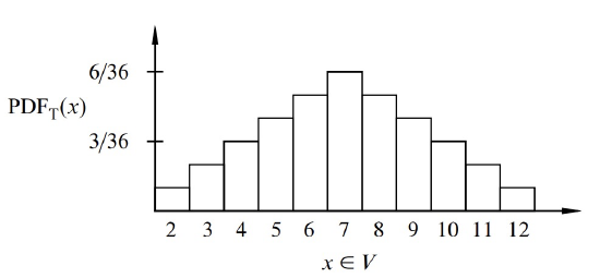
As an example, suppose that you roll two unbiased, independent, 6-sided dice. Let \(T\) be the random variable that equals the sum of the two rolls. This random variable takes on values in the set \(V = \{2, 3, \ldots, 12\}\). A plot of the probability density function for \(T\) is shown in Figure 18.1. The lump in the middle indicates that sums close to 7 are the most likely. The total area of all the rectangles is 1 since the dice must take on exactly one of the sums in \(V = \{2, 3, \ldots, 12\}\).
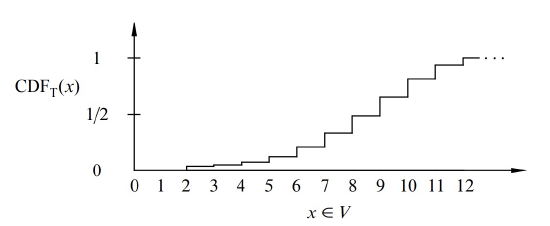
The cumulative distribution function for \(T\) is shown in Figure 18.2: The height of the \(i\)th bar in the cumulative distribution function is equal to the sum of the heights of the leftmost \(i\) bars in the probability density function. This follows from the definitions of pdf and cdf:
\[\nonumber \text{CDF}_R (x) = \text{Pr}[R \leq x] = \sum_{y \leq x} \text{Pr}[R = y] = \sum_{y \leq x} \text{PDF}_R (y).\]
It also follows from the definition that
\[\nonumber \lim_{x \rightarrow \infty} \text{CDF}_R (x) = 1 \text{ and } \lim_{x \rightarrow -\infty} \text{CDF}_R (x) = 0.\]
Both \(\text{PDF}_R\) and \(\text{CDF}_R\) capture the same information about \(R\), so take your choice. The key point here is that neither the probability density function nor the cumulative distribution function involves the sample space of an experiment.
One of the really interesting things about density functions and distribution functions is that many random variables turn out to have the same pdf and cdf. In other words, even though \(R\) and \(S\) are different random variables on different probability spaces, it is often the case that
\[\nonumber \text{PDF}_R = \text{PDF}_S.\]
In fact, some pdf’s are so common that they are given special names. For example, the three most important distributions in computer science are the Bernoulli distribution, the uniform distribution, and the binomial distribution. We look more closely at these common distributions in the next several sections.
Bernoulli Distributions
A Bernoulli distribution is the distribution function for a Bernoulli variable. Specifically, the Bernoulli distribution has a probability density function of the form \(f_p : \{0, 1\} \rightarrow [0, 1]\) where
\[\begin{aligned} f_p(0) &= p, \text{ and } \\ f_p(1) &= 1 - p, \end{aligned}\]
for some \(p \in [0, 1]\). The corresponding cumulative distribution function is \(F_p : \mathbb{R} \rightarrow [0, 1]\) where
\[\nonumber F_p(x) ::=\left\{\begin{array}{ll} 0 & \text { if } x < 0 \\ p & \text { if } 0 \leq x \leq 1 \\ 1 & \text { if } 1 \leq x \end{array}\right.\]
Uniform Distributions
A random variable that takes on each possible value in its codomain with the same probability is said to be uniform. If the codomain \(V\) has \(n\) elements, then the uniform distribution has a pdf of the form
\[\nonumber f : V \rightarrow [0, 1]\]
where
\[\nonumber f(v) = \frac{1}{n}\]
for all \(v \in V.\)
If the elements of \(V\) in increasing order are \(a_1, a_2, \ldots,a_n\), then the cumulative distribution function would be \(F : \mathbb{R} \rightarrow [0,1]\) where
\[\nonumber F(x) ::=\left\{\begin{array}{ll} 0 & \text { if } x < a_1 \\ k/n & \text { if } a_k \leq x \leq a_{k+1} \text{ for } 1 \leq k < n \\ 1 & \text { if } a_n \leq x. \end{array}\right.\]
Uniform distributions come up all the time. For example, the number rolled on a fair die is uniform on the set \(\{1, 2, \ldots, 6\}\). An indicator variable is uniform when its pdf is \(f_{1/2}\).
The Numbers Game
Enough definitions—let’s play a game! We have two envelopes. Each contains an integer in the range \(0, 1, \ldots, 100\), and the numbers are distinct. To win the game, you must determine which envelope contains the larger number. To give you a fighting chance, we’ll let you peek at the number in one envelope selected at random. Can you devise a strategy that gives you a better than 50% chance of winning?
For example, you could just pick an envelope at random and guess that it contains the larger number. But this strategy wins only 50% of the time. Your challenge is to do better.
So you might try to be more clever. Suppose you peek in one envelope and see the number 12. Since 12 is a small number, you might guess that the number in the other envelope is larger. But perhaps we’ve been tricky and put small numbers in both envelopes. Then your guess might not be so good!
An important point here is that the numbers in the envelopes may not be random. We’re picking the numbers and we’re choosing them in a way that we think will defeat your guessing strategy. We’ll only use randomization to choose the numbers if that serves our purpose: making you lose!
Intuition Behind the Winning Strategy
People are surprised when they first learn that there is a strategy that wins more than 50% of the time, regardless of what numbers we put in the envelopes.
Suppose that you somehow knew a number \(x\) that was in between the numbers in the envelopes. Now you peek in one envelope and see a number. If it is bigger than \(x\), then you know you’re peeking at the higher number. If it is smaller than \(x\), then you’re peeking at the lower number. In other words, if you know a number \(x\) between the numbers in the envelopes, then you are certain to win the game.
The only flaw with this brilliant strategy is that you do not know such an \(x\). This sounds like a dead end, but there’s a cool way to salvage things: try to guess \(x\)! There is some probability that you guess correctly. In this case, you win 100% of the time. On the other hand, if you guess incorrectly, then you’re no worse off than before; your chance of winning is still 50%. Combining these two cases, your overall chance of winning is better than 50%.
Many intuitive arguments about probability are wrong despite sounding persuasive. But this one goes the other way: it may not convince you, but it’s actually correct. To justify this, we’ll go over the argument in a more rigorous way—and while we’re at it, work out the optimal way to play.
Analysis of the Winning Strategy
For generality, suppose that we can choose numbers from the integer interval \([0..n]\). Call the lower number \(L\) and the higher number \(H\).
Your goal is to guess a number \(x\) between \(L\) and \(H\). It’s simplest if \(x\) does not equal \(L\) or \(H\), so you should select \(x\) at random from among the half-integers:
\[\nonumber \frac{1}{2}, \frac{3}{2}, \frac{5}{2}, \cdots, \frac{2n - 1}{2}\]
But what probability distribution should you use?
The uniform distribution—selecting each of these half-integers with equal probability— turns out to be your best bet. An informal justification is that if we figured out that you were unlikely to pick some number—say \(50 \frac{1}{2}\)—then we’d always put 50 and 51 in the envelopes. Then you’d be unlikely to pick an \(x\) between \(L\) and \(H\) and would have less chance of winning.
After you’ve selected the number \(x\), you peek into an envelope and see some number \(T\). If \(T > x\), then you guess that you’re looking at the larger number. If \(T < x\), then you guess that the other number is larger.
All that remains is to determine the probability that this strategy succeeds. We can do this with the usual four step method and a tree diagram.
Step 1: Find the sample space.
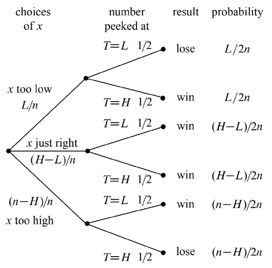
You either choose x too low \((< L)\), too high \((> H)\), or just right \((L < x < H)\). Then you either peek at the lower number \((T = L)\) or the higher number \((T = H)\). This gives a total of six possible outcomes, as show in Figure 18.3.
Step 2: Define events of interest.
The four outcomes in the event that you win are marked in the tree diagram.
Step 3: Assign outcome probabilities.
First, we assign edge probabilities. Your guess \(x\) is too low with probability \(L/n\), too high with probability \((n - H)/n\), and just right with probability \((H - L)/n\). Next, you peek at either the lower or higher number with equal probability. Multiplying along root-to-leaf paths gives the outcome probabilities.
Step 4: Compute event probabilities.
The probability of the event that you win is the sum of the probabilities of the four outcomes in that event:
\[\begin{aligned} \text{Pr}[\text{win}] &= \frac{L}{2n} + \frac{H - L}{2n} + \frac{H - L}{2n} + \frac{n - H}{2n} \\ &= \frac{1}{2} + \frac{H - L}{2n} \\ &\geq \frac{1}{2} + \frac{1}{2n} \end{aligned}\]
The final inequality relies on the fact that the higher number \(H\) is at least 1 greater than the lower number \(L\) since they are required to be distinct.
Sure enough, you win with this strategy more than half the time, regardless of the numbers in the envelopes! So with numbers chosen from the range \(0, 1, \ldots, 100\), you win with probability at least \(1/2 + 1/200 = 50.5\%\). If instead we agree to stick to numbers \(0, 1, \ldots, 10\), then your probability of winning rises to 55%. By Las Vegas standards, those are great odds.
Randomized Algorithms
The best strategy to win the numbers game is an example of a randomized algorithm—it uses random numbers to influence decisions. Protocols and algorithms that make use of random numbers are very important in computer science. There are many problems for which the best known solutions are based on a random number generator.
For example, the most commonly-used protocol for deciding when to send a broadcast on a shared bus or Ethernet is a randomized algorithm known as exponential backoff. One of the most commonly-used sorting algorithms used in practice, called quicksort, uses random numbers. You’ll see many more examples if you take an algorithms course. In each case, randomness is used to improve the probability that the algorithm runs quickly or otherwise performs well.
Binomial Distributions
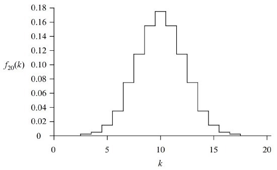
The third commonly-used distribution in computer science is the binomial distribution. The standard example of a random variable with a binomial distribution is the number of heads that come up in \(n\) independent flips of a coin. If the coin is fair, then the number of heads has an unbiased binomial distribution, specified by the pdf \(f_n : [0..n] \rightarrow [0, 1]\):
\[\nonumber f_n(k) ::= {n \choose k} 2^{-n}.\]
This is because there are \({n \choose k}\) sequences of \(n\) coin tosses with exactly \(k\) heads, and each such sequence has probability \(2^{-n}\).
A plot of \(f_{20}(k)\) is wn in Figure 18.4. The most likely outcome is \(k = 10\) heads, and the probability falls off rapidly for larger and smaller values of \(k\). The falloff regions to the left and right of the main hump are called the tails of the distribution.
In many fields, including Computer Science, probability analyses come down to getting small bounds on the tails of the binomial distribution. In the context of a problem, this typically means that there is very small probability that something bad happens, which could be a server or communication link overloading or a randomized algorithm running for an exceptionally long time or producing the wrong result.
The tails do get small very fast. For example, the probability of flipping at most 25 heads in 100 tosses is less than 1 in 3,000,000. In fact, the tail of the distribution falls off so rapidly that the probability of flipping exactly 25 heads is nearly twice the probability of flipping exactly 24 heads plus the probability of flipping exactly 23 heads plus ... the probability of flipping no heads.
The General Binomial Distribution
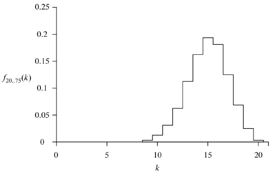
If the coins are biased so that each coin is heads with probability \(p\), then the number of heads has a general binomial density function specified by the pdf \(f_{n, p} : [0..n] \rightarrow [0, 1]\) where
\[f_{n, p}(k) = {n \choose k}p^k (1-p)^{n-k}.\]
for some \(n \in \mathbb{N}^+\) and \(p \in [0, 1]\). This is because there are \({n \choose k}\) sequences with \(k\) heads and \(n - k\) tails, but now \(p^k (1-p)^{n-k}\) is the probability of each such sequence.
For example, the plot in Figure 18.5 shows the probability density function \(f_{n,p}(k)\) corresponding to flipping \(n = 20\) independent coins that are heads with probability \(p = 0.75\). The graph shows that we are most likely to get \(k = 15\) heads, as you might expect. Once again, the probability falls off quickly for larger and smaller values of \(k\).