18.4: Great Expectations

The expectation or expected value of a random variable is a single number that reveals a lot about the behavior of the variable. The expectation of a random variable is also known as its mean or average. For example, the first thing you typically want to know when you see your grade on an exam is the average score of the class. This average score turns out to be precisely the expectation of the random variable equal to the score of a random student.

More precisely, the expectation of a random variable is its “average” value when each value is weighted according to its probability. Formally, the expected value of a random variable is defined as follows:

Definition \(\PageIndex{1}\)

If \(R\) is a random variable defined on a sample space \(S\), then the expectation of \(R\) is

\[\label{18.4.1} \text{Ex}[R] ::= \sum_{\omega \in S} R(\omega)\text{Pr}[\omega].\]

Let’s work through some examples.

The Expected Value of a Uniform Random Variable

Rolling a 6-sided die provides an example of a uniform random variable. Let \(R\) be the value that comes up when you roll a fair 6-sided die. Then by (\ref{18.4.1}), the expected value of \(R\) is

\[\nonumber \text{Ex}[R] = 1 \cdot \frac{1}{6} + 2 \cdot \frac{1}{6} + 3 \cdot \frac{1}{6} + 4 \cdot \frac{1}{6} + 5 \cdot \frac{1}{6} + 6 \cdot \frac{1}{6} = \frac{7}{2}.\]

This calculation shows that the name “expected” value is a little misleading; the random variable might never actually take on that value. No one expects to roll a \(3\frac{1}{2}\) on an ordinary die!

In general, if \(R_n\) is a random variable with a uniform distribution on \(\{a_1, a_2, \ldots, a_n\}\), then the expectation of \(R_n\) is simply the average of the \(a_i\)’s:

\[\nonumber \text{Ex}[R_n] = \frac{a_1 +a_2 + \cdots + a_n}{n}.\]

The Expected Value of a Reciprocal Random Variable

Define a random variable \(S\) to be the reciprocal of the value that comes up when you roll a fair 6-sided die. That is, \(S = 1/R\) where \(R\) is the value that you roll. Now,

\[\nonumber \text{Ex}[S] = \text{Ex}\left[\frac{1}{R}\right] = \frac{1}{1} \cdot \frac{1}{6} + \frac{1}{2} \cdot \frac{1}{6} + \frac{1}{3} \cdot \frac{1}{6} + \frac{1}{4} \cdot \frac{1}{6} + \frac{1}{5} \cdot \frac{1}{6} + \frac{1}{6} \cdot \frac{1}{6} = \frac{49}{120}.\]

Notice that

\[\nonumber \text{Ex}[1/R] \neq 1 / \text{Ex}[R].\]

The Expected Value of an Indicator Random Variable

The expected value of an indicator random variable for an event is just the probability of that event.

Lemma 18.4.2. If \(I_A\) is the indicator random variable for event \(A\), then

\[\nonumber \text{Ex}[I_A] = \text{Pr}[A].\]

Proof.

\[\begin{aligned} \text{Ex}[I_A] = 1 \cdot \text{Pr}[I_A = 1] + 0 \cdot \text{Pr}[I_A = 0] &= \text{Pr}[I_A = 1] \\ &= \text{Pr}[A]. & (\text{def of } I_A) \end{aligned}\]

For example, if \(A\) is the event that a coin with bias \(p\) comes up heads, then \(\text{Ex}[I_A] = \text{Pr}[I_A = 1] = p\).

Alternate Definition of Expectation

There is another standard way to define expectation.

Theorem \(\PageIndex{3}\)

For any random variable \(R\),

\[\label{18.4.2} \text{Ex}[R] = \sum_{x \in \text{ range}(R)} x \cdot \text{Pr}[R = x].\]

The proof of Theorem 18.4.3, like many of the elementary proofs about expectation in this chapter, follows by regrouping of terms in equation (\ref{18.4.1}):

Proof

Suppose \(R\) is defined on a sample space \(S\). Then,

\[\begin{aligned} \text{Ex}[R] &::= \sum_{\omega \in S} R(\omega)\text{Pr}[\omega] \\ &= \sum_{x \in \text{ range}(R)} \sum_{x \in [R = x]} R(\omega)\text{Pr}[\omega] \\ &= \sum_{x \in \text{ range}(R)} \sum_{x \in [R = x]} x \text{Pr}[\omega] & (\text{def of the event }[R = x]) \\ &= \sum_{x \in \text{ range}(R)} x \left(\sum_{x \in [R = x]} \text{Pr}[\omega]\right) & (\text{factoring } x \text{ from the inner sum}) \\ &= \sum_{x \in \text{ range}(R)} x \cdot \text{Pr}[R = x]. & (\text{def of Pr}[R = x]) \end{aligned}\]

The first equality follows because the events \([R = x]\) for \(x \in \text{range}(R)\) partition the sample space \(S\), so summing over the outcomes in \([R = x]\) for \(x \in \text{range}(R)\) is the same as summing over \(S\). \(\quad \blacksquare\)

In general, equation (\ref{18.4.2}) is more useful than the defining equation (\ref{18.4.1}) for calculating expected values. It also has the advantage that it does not depend on the sample space, but only on the density function of the random variable. On the other hand, summing over all outcomes as in equation (\ref{18.4.1}) sometimes yields easier proofs about general properties of expectation.

Conditional Expectation

Just like event probabilities, expectations can be conditioned on some event. Given a random variable \(R\), the expected value of \(R\) conditioned on an event \(A\) is the probability-weighted average value of R over outcomes in \(A\). More formally:

Definition \(\PageIndex{4}\)

The conditional expectation \(\text{Ex}[R \mid A]\) of a random variable \(R\) given event \(A\) is:

\[\label{18.4.3} \text{Ex}[R \mid A] ::= \sum_{r \in \text{ range}(R)} r \cdot \text{Pr}[R = r \mid A].\]

For example, we can compute the expected value of a roll of a fair die, given that the number rolled is at least 4. We do this by letting \(R\) be the outcome of a roll of the die. Then by equation (\ref{18.4.3}),

\[\nonumber \text{Ex}[R \mid R \geq 4] = \sum_{i = 1}^{6} i \cdot \text{Pr}[R = i \mid R \geq 4] = 1\cdot 0 + 2 \cdot 0 +3 \cdot 0 + 4 \cdot \frac{1}{3} + 5 \cdot \frac{1}{3} + 6 \cdot \frac{1}{3} = 5.\]

Conditional expectation is useful in dividing complicated expectation calculations into simpler cases. We can find a desired expectation by calculating the conditional expectation in each simple case and averaging them, weighing each case by its probability.

For example, suppose that 49.6% of the people in the world are male and the rest female—which is more or less true. Also suppose the expected height of a randomly chosen male is \(5' 11''\), while the expected height of a randomly chosen female is \(5' 5''\) What is the expected height of a randomly chosen person? We can calculate this by averaging the heights of men and women. Namely, let \(H\) be the height (in feet) of a randomly chosen person, and let \(M\) be the event that the person is male and \(F\) the event that the person is female. Then

\[\begin{aligned} \text{Ex}[H] &= \text{Ex}[H \mid M] \text{Pr}[M] + \text{Ex}[H \mid F] \text{Pr}[F] \\ &= (5 + 11/12) \cdot 0.496 + (5 + 5/12) \cdot (1 - 0.496) \\ &= 5.6646 \cdots \end{aligned}\]

which is a little less than \(5' 8''.\)

This method is justified by:

Theorem \(\PageIndex{5}\)

(Law of Total Expectation). Let \(R\) be a random variable on a sample space \(S\), and suppose that \(A_1, A_2, \ldots ,\) is a partition of \(S\). Then

\[\nonumber \text{Ex}[R] = \sum_{i} \text{Ex}[R \mid A_i] \text{Pr}[A_i].\]

Proof

\[\begin{aligned} \text{Ex}[R] &= \sum_{r \in \text{range}(R)} r \cdot \text{Pr}[R = r] & (\text{by 18.4.2}) \\ &= \sum_{r} r \cdot \sum_{i} \text{Pr}[R = r \mid A_i] \text{Pr}[A_i] & (\text{Law of Total Probability}) \\ &= \sum_{r}\sum_{i} r \cdot \text{Pr}[R = r \mid A_i] \text{Pr}[A_i] & (\text{distribute constant } r) \\ &= \sum_{i}\sum_{r} r \cdot \text{Pr}[R = r \mid A_i] \text{Pr}[A_i] & (\text{exchange order of summation}) \\ &= \sum_{i} \text{Pr}[A_i] \sum_{r} r \cdot \text{Pr}[R = r \mid A_i] & (\text{factor constant Pr}[A_i]) \\ &= \sum_{i} \text{Pr}[A_i] \text{Ex}[R \mid A_i]. & (\text{Def 18.4.4 of cond. expectation}) \\ & & \quad \blacksquare \end{aligned}\]

Mean Time to Failure

A computer program crashes at the end of each hour of use with probability \(p\), if it has not crashed already. What is the expected time until the program crashes? This will be easy to figure out using the Law of Total Expectation, Theorem 18.4.5. Specifically, we want to find \(\text{Ex}[C]\) where \(C\) is the number of hours until the first crash. We’ll do this by conditioning on whether or not the crash occurs in the first hour.

So define \(A\) to be the event that the system fails on the first step and \(\overline{A}\) to be the complementary event that the system does not fail on the first step. Then the mean time to failure \(\text{Ex}[C]\) is

\[\label{18.4.4} \text{Ex}[C] = \text{Ex}[C \mid A] \text{Pr}[A] + \text{Ex}[C \mid \overline{A}] \text{Pr}[\overline{A}].\]

Since \(A\) is the condition that the system crashes on the first step, we know that

\[\label{18.4.5} \text{Ex}[C \mid A] = 1.\]

Since \(\overline{A}\) is the condition that the system does not crash on the first step, conditioning on \(\overline{A}\) is equivalent to taking a first step without failure and then starting over without conditioning. Hence,

\[\label{18.4.6} \text{Ex}[C \mid \overline{A}] = 1 + \text{Ex}[C].\]

Plugging (\ref{18.4.5}) and (\ref{18.4.6}) into (\ref{18.4.4}):

\[\begin{aligned} \text{Ex}[C] &= 1 \cdot p + (1 + \text{Ex}[C])(1 - p) \\ &= p + 1 - p + (1 - p)\text{Ex}[C] \\ &= 1 + (1 - p)\text{Ex}[C]. \end{aligned}\]

Then, rearranging terms gives

\[\nonumber 1 = \text{Ex}[C] - (1 - p)\text{Ex}[C] = p\text{Ex}[C],\]

and thus

\[\nonumber \text{Ex}[C] = 1/p.\]

The general principle here is well-worth remembering.

Mean Time to Failure

If a system independently fails at each time step with probability \(p\), then the expected number of steps up to the first failure is \(1/p\).

So, for example, if there is a 1% chance that the program crashes at the end of each hour, then the expected time until the program crashes is \(1/0.01 = 100\) hours.

As a further example, suppose a couple insists on having children until they get a boy, then how many baby girls should they expect before their first boy? Assume for simplicity that there is a 50% chance that a child will be a boy and that the genders of siblings are mutually independent.

This is really a variant of the previous problem. The question, “How many hours until the program crashes?” is mathematically the same as the question, “How many children must the couple have until they get a boy?” In this case, a crash corresponds to having a boy, so we should set \(p = 1/2\). By the preceding analysis, the couple should expect a baby boy after having \(1/p = 2\) children. Since the last of these will be a boy, they should expect just one girl. So even in societies where couples pursue this commitment to boys, the expected population will divide evenly between boys and girls.

There is a simple intuitive argument that explains the mean time to failure formula (\ref{18.4.7}). Suppose the system is restarted after each failure. This makes the mean time to failure the same as the mean time between successive repeated failures. Now if the probability of failure at a given step is \(p\), then after \(n\) steps we expect to have \(pn\) failures. Now, by definition, the average number of steps between failures is equal to \(np/p\), namely, \(1/p\).

For the record, we’ll state a formal version of this result. A random variable like \(C\) that counts steps to first failure is said to have a geometric distribution with parameter \(p\).

Definition \(\PageIndex{6}\)

A random variable, \(C\), has a geometric distribution with parameter \(p\) iff \(\text{codomain}(C) = \mathbb{Z}^+\) and

\[\nonumber \text{Pr}[C = i] = (1 - p)^{i - 1} p.\]

Lemma 18.4.7. If a random variable \(C\) has a geometric distribution with parameter \(p\), then

\[\label{18.4.7} \text{Ex}[C] = \frac{1}{p}.\]

Expected Returns in Gambling Games

Some of the most interesting examples of expectation can be explained in terms of gambling games. For straightforward games where you win \(w\) dollars with probability \(p\) and you lose \(x\) dollars with probability \(1 - p\), it is easy to compute your expected return or winnings. It is simply

\[\nonumber pw - (1 - p)x \text{ dollars}.\]

For example, if you are flipping a fair coin and you win $1 for heads and you lose $1 for tails, then your expected winnings are

\[\nonumber \frac{1}{2} \cdot 1 - \left( 1 - \frac{1}{2}\right) \cdot 1 = 0.\]

In such cases, the game is said to be fair since your expected return is zero.

Splitting the Pot

We’ll now look at a different game which is fair—but only on first analysis.

It’s late on a Friday night in your neighborhood hangout when two new biker dudes, Eric and Nick, stroll over and propose a simple wager. Each player will put $2 on the bar and secretly write “heads” or “tails” on their napkin. Then you will flip a fair coin. The $6 on the bar will then be “split”—that is, be divided equally—among the players who correctly predicted the outcome of the coin toss. Pot splitting like this is a familiar feature in poker games, betting pools, and lotteries.

This sounds like a fair game, but after your regrettable encounter with strange dice (Section 16.3), you are definitely skeptical about gambling with bikers. So before agreeing to play, you go through the four-step method and write out the tree diagram to compute your expected return. The tree diagram is shown in Figure 18.6.

Figure 18.6 The tree diagram for the game where three players each wager $2 and then guess the outcome of a fair coin toss. The winners split the pot.

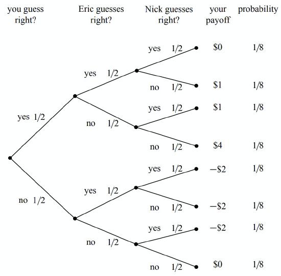
The “payoff” values in Figure 18.6 are computed by dividing the $6 pot¹ among those players who guessed correctly and then subtracting the $2 that you put into the pot at the beginning. For example, if all three players guessed correctly, then your payoff is $0, since you just get back your $2 wager. If you and Nick guess correctly and Eric guessed wrong, then your payoff is

\[\nonumber \frac{6}{2} - 2 = 1.\]

In the case that everyone is wrong, you all agree to split the pot and so, again, your payoff is zero.

To compute your expected return, you use equation (\ref{18.4.2}):

\[\begin{aligned} \text{Ex[playoff]} &= 0 \cdot \frac{1}{8} + 1 \cdot \frac{1}{8} + 1 \cdot \frac{1}{8} + 4 \cdot \frac{1}{8} + (-2) \cdot \frac{1}{8} + (-2) \cdot \frac{1}{8} + (-2) \cdot \frac{1}{8} + 0 \cdot \frac{1}{8} \\ &= 0.\end{aligned}\]

This confirms that the game is fair. So, for old time’s sake, you break your solemn vow to never ever engage in strange gambling games.

The Impact of Collusion

Needless to say, things are not turning out well for you. The more times you play the game, the more money you seem to be losing. After 1000 wagers, you have lost over $500. As Nick and Eric are consoling you on your “bad luck,” you do a back-of-the-envelope calculation and decide that the probability of losing $500 in 1000 fair $2 wagers is very, very small.

Now it is possible of course that you are very, very unlucky. But it is more likely that something fishy is going on. Somehow the tree diagram in Figure 18.6 is not a good model of the game.

The “something” that’s fishy is the opportunity that Nick and Eric have to collude against you. The fact that the coin flip is fair certainly means that each of Nick and Eric can only guess the outcome of the coin toss with probability \(1/2\). But when you look back at the previous 1000 bets, you notice that Eric and Nick never made the same guess. In other words, Nick always guessed “tails” when Eric guessed “heads,” and vice-versa. Modelling this fact now results in a slightly different tree diagram, as shown in Figure 18.7.

Figure 18.7 The revised tree diagram reflecting the scenario where Nick always guesses the opposite of Eric.

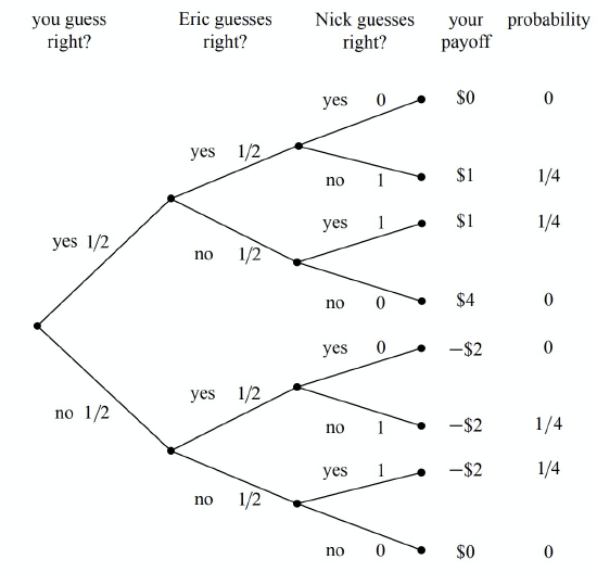
The payoffs for each outcome are the same in Figures 18.6 and 18.7, but the probabilities of the outcomes are different. For example, it is no longer possible for all three players to guess correctly, since Nick and Eric are always guessing differently. More importantly, the outcome where your payoff is $4 is also no longer possible. Since Nick and Eric are always guessing differently, one of them will always get a share of the pot. As you might imagine, this is not good for you!

When we use equation (\ref{18.4.2}) to compute your expected return in the collusion scenario, we find that

\[\begin{aligned} \text{Ex[playoff]} &= 0 \cdot 0 + 1 \cdot \frac{1}{4} + 1 \cdot \frac{1}{4} + 4 \cdot 0 + (-2) \cdot 0 + (-2) \cdot \frac{1}{4} + (-2) \cdot \frac{1}{4} + 0 \cdot - \\ &= - \frac{1}{2}. \end{aligned}\]

So watch out for these biker dudes! By colluding, Nick and Eric have made it so that you expect to lose $.50 every time you play. No wonder you lost $500 over the course of 1000 wagers.

How to Win the Lottery

Similar opportunities to collude arise in many betting games. For example, consider the typical weekly football betting pool, where each participant wagers $10 and the participants that pick the most games correctly split a large pot. The pool seems fair if you think of it as in Figure 18.6. But, in fact, if two or more players collude by guessing differently, they can get an “unfair” advantage at your expense!

In some cases, the collusion is inadvertent and you can profit from it. For example, many years ago, a former MIT Professor of Mathematics named Herman Chernoff figured out a way to make money by playing the state lottery. This was surprising since the state usually takes a large share of the wagers before paying the winners, and so the expected return from a lottery ticket is typically pretty poor. So how did Chernoff find a way to make money? It turned out to be easy!

In a typical state lottery,

• all players pay $1 to play and select 4 numbers from 1 to 36,
• the state draws 4 numbers from 1 to 36 uniformly at random,
• the states divides \(1/2\) of the money collected among the people who guessed correctly and spends the other half redecorating the governor’s residence.

This is a lot like the game you played with Nick and Eric, except that there are more players and more choices. Chernoff discovered that a small set of numbers was selected by a large fraction of the population. Apparently many people think the same way; they pick the same numbers not on purpose as in the previous game with Nick and Eric, but based on the Red Sox winning average or today’s date. The result is as though the players were intentionally colluding to lose. If any one of them guessed correctly, then they’d have to split the pot with many other players. By selecting numbers uniformly at random, Chernoff was unlikely to get one of these favored sequences. So if he won, he’d likely get the whole pot! By analyzing actual state lottery data, he determined that he could win an average of 7 cents on the dollar. In other words, his expected return was not \(-$.50\) as you might think, but \(+$.07\). ² Inadvertent collusion often arises in betting pools and is a phenomenon that you can take advantage of.

¹The money invested in a wager is commonly referred to as the pot.

²Most lotteries now offer randomized tickets to help smooth out the distribution of selected sequences.