19.2: Chebyshev’s Theorem

We’ve seen that Markov’s Theorem can give a better bound when applied to \(R - b\) rather than \(R\). More generally, a good trick for getting stronger bounds on a random variable \(R\) out of Markov’s Theorem is to apply the theorem to some cleverly chosen function of \(R\). Choosing functions that are powers of the absolute value of R turns out to be especially useful. In particular, since \(|R|^{z}\) is nonnegative for any real number \(z\), Markov’s inequality also applies to the event \([|R|^{z} \geq x^z]\). But for positive \(x, z\) > 0 this event is equivalent to the event \([|R| \geq x]\) for , so we have:

Lemma 19.2.1. For any random variable \(R\) and positive real numbers \(x, z\),

\[\nonumber \text{Pr}[|R| \geq x] \leq \frac{\text{Ex}[|R|^z]}{x^z}.\]

Rephrasing (19.2.1) in terms of \(|R - \text{Ex}[R]|\), the random variable that measures R’s deviation from its mean, we get

\[\label{19.2.1} \text{Pr}[|R - \text{Ex}[R]|\geq x] \leq \frac{\text{Ex}[(R - \text{Ex}[R])^z]}{x^z}.\]

The case when \(z = 2\) turns out to be so important that the numerator of the right hand side of (\ref{19.2.1}) has been given a name:

Definition \(\PageIndex{2}\)

The variance, \(\text{Var}[R]\), of a random variable, \(R\), is:

\[\nonumber \text{Var}[R] ::= \text{Ex}[(R - \text{Ex}[R])^2].\]

Variance is also known as mean square deviation.

The restatement of (\ref{19.2.1}) for \(z = 2\) is known as Chebyshev’s Theorem¹

Theorem \(\PageIndex{3}\)

(Chebyshev). Let \(R\) be a random variable and \(x \in \mathbb{R}^+\). Then

\[\nonumber \text{Pr}[|R - \text{Ex}[R]| \geq x ] \leq \frac{\text{Var}[R]}{x^2}.\]

The expression \(\text{Ex}[(R - \text{Ex}[R])^2]\) for variance is a bit cryptic; the best approach is to work through it from the inside out. The innermost expression, \(R - \text{Ex}[R]\), is precisely the deviation of \(R\) above its mean. Squaring this, we obtain, \((R - \text{Ex}[R])^2\). This is a random variable that is near 0 when \(R\) is close to the mean and is a large positive number when \(R\) deviates far above or below the mean. So if \(R\) is always close to the mean, then the variance will be small. If \(R\) is often far from the mean, then the variance will be large.

Variance in Two Gambling Games

The relevance of variance is apparent when we compare the following two gambling games.

Game A: We win $2 with probability \(2/3\) and lose $1 with probability \(1/3\).

Game B: We win $1002 with probability \(2/3\) and lose $2001 with probability \(1/3\).

Which game is better financially? We have the same probability, \(2/3\), of winning each game, but that does not tell the whole story. What about the expected return for each game? Let random variables \(A\) and \(B\) be the payoffs for the two games. For example, \(A\) is 2 with probability \(2/3\) and -1 with probability \(1/3\). We can compute the expected payoff for each game as follows:

\[\nonumber \text{Ex}[A] = 2 \cdot \frac{2}{3} + (-1) \cdot \frac{1}{3} = 1,\]

\[\nonumber \text{Ex}[B] = 1002 \cdot \frac{2}{3} + (-2001) \cdot \frac{1}{3} = 1.\]

The expected payoff is the same for both games, but the games are very different. This difference is not apparent in their expected value, but is captured by variance.

We can compute the \(\text{Var}[A]\) by working “from the inside out” as follows:

\[\begin{aligned} A - \text{Ex}[A] &=\left\{\begin{array}{ll} 1 & \text { with probability } \frac{2}{3} \\ -2 & \text { with probability } \frac{1}{3} \end{array}\right. \\ (A - \text{Ex}[A])^2 &=\left\{\begin{array}{ll} 1 & \text { with probability } \frac{2}{3} \\ 4 & \text { with probability } \frac{1}{3} \end{array}\right. \\ \text{Ex}[(A - \text{Ex}[A])^2] &= 1 \cdot \frac{2}{3} + 4 \cdot \frac{1}{3} \\ \text{Var}[A] &= 2. \end{aligned}\]

Similarly, we have for \(\text{Var}[B]\):

\[\begin{aligned} B - \text{Ex}[B] &=\left\{\begin{array}{ll} 1001 & \text { with probability } \frac{2}{3} \\ -2002 & \text { with probability } \frac{1}{3} \end{array}\right. \\ (B - \text{Ex}[B])^2 &=\left\{\begin{array}{ll} 1,002,001 & \text { with probability } \frac{2}{3} \\ 4,008,004 & \text { with probability } \frac{1}{3} \end{array}\right. \\ \text{Ex}[(B - \text{Ex}[B])^2] &= 1,002,001 \cdot \frac{2}{3} + 4,008,004 \cdot \frac{1}{3} \\ \text{Var}[B] &= 2,004,002. \end{aligned}\]

The variance of Game A is 2 and the variance of Game B is more than two million! Intuitively, this means that the payoff in Game A is usually close to the expected value of $1, but the payoff in Game B can deviate very far from this expected value.

High variance is often associated with high risk. For example, in ten rounds of Game A, we expect to make $10, but could conceivably lose $10 instead. On the other hand, in ten rounds of game B, we also expect to make $10, but could actually lose more than $20,000!

Standard Deviation

In Game B above, the deviation from the mean is 1001 in one outcome and -2002 in the other. But the variance is a whopping 2,004,002. The happens because the “units” of variance are wrong: if the random variable is in dollars, then the expectation is also in dollars, but the variance is in square dollars. For this reason, people often describe random variables using standard deviation instead of variance.

Definition \(\PageIndex{4}\)

The standard deviation, \(\sigma_R\), of a random variable, \(R\), is the square root of the variance:

\[\nonumber \sigma_R ::= \sqrt{\text{Var}[R]} = \sqrt{\text{Ex}[(R - \text{Ex}[R])^2]}.\]

So the standard deviation is the square root of the mean square deviation, or the root mean square for short. It has the same units—dollars in our example—as the original random variable and as the mean. Intuitively, it measures the average deviation from the mean, since we can think of the square root on the outside as canceling the square on the inside.

Example 19.2.5. The standard deviation of the payoff in Game B is:

\[\nonumber \sigma_R = \sqrt{\text{Var}[B]} = \sqrt{2,004,002} \approx 1416.\]

The random variable \(B\) actually deviates from the mean by either positive 1001 or negative 2002, so the standard deviation of 1416 describes this situation more closely than the value in the millions of the variance.

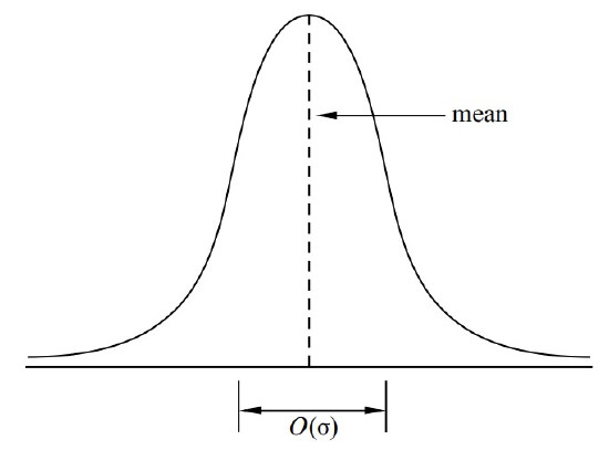
For bell-shaped distributions like the one illustrated in Figure 19.1, the standard deviation measures the “width” of the interval in which values are most likely to fall. This can be more clearly explained by rephrasing Chebyshev’s Theorem in terms of standard deviation, which we can do by substituting \(x = c \sigma_R\) in (19.1):

Figure 19.1 The standard deviation of a distribution indicates how wide the “main part” of it is.

Corollary 19.2.6. Let \(R\) be a random variable, and let \(c\) be a positive real number.

\[\text{Pr}[|R - \text{Ex}[R]| \geq c \sigma_R] \leq \frac{1}{c^2}.\]

Now we see explicitly how the “likely” values of \(R\) are clustered in an \(O(\sigma_R)\)-sized region around \(\text{Ex}[R]\), confirming that the standard deviation measures how spread out the distribution of \(R\) is around its mean.

The IQ Example

Suppose that, in addition to the national average IQ being 100, we also know the standard deviation of IQ’s is 10. How rare is an IQ of 300 or more?

Let the random variable, \(R\), be the IQ of a random person. So \(\text{Ex}[R] = 100\), \(\sigma_R = 10\), and \(R\) is nonnegative. We want to compute \(\text{Pr}[R \geq 300]\).

We have already seen that Markov’s Theorem 19.1.1 gives a coarse bound, namely,

\[\nonumber \text{Pr}[R \geq 300] \leq \frac{1}{3}.\]

Now we apply Chebyshev’s Theorem to the same problem:

\[\nonumber \text{Pr}[R \geq 300] = \text{Pr}[|R - 100| \geq 200] \leq \frac{\text{Var}[R]}{200^2} = \frac{10^2}{200^2} = \frac{1}{400}.\]

So Chebyshev’s Theorem implies that at most one person in four hundred has an IQ of 300 or more. We have gotten a much tighter bound using additional information—the variance of \(R\)—than we could get knowing only the expectation.

¹There are Chebyshev Theorems in several other disciplines, but Theorem 19.2.3 is the only one we’ll refer to.