20.1: Gambler’s Ruin

Suppose a gambler starts with an initial stake of \(n\) dollars and makes a sequence of $1 bets. If he wins an individual bet, he gets his money back plus another $1. If he loses the bet, he loses the $1.

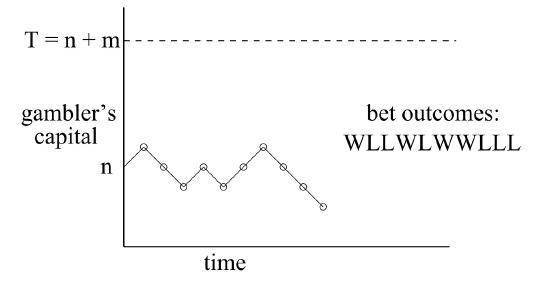
We can model this scenario as a random walk between integer points on the real line. The position on the line at any time corresponds to the gambler’s cash-onhand, or capital. Walking one step to the right corresponds to winning a $1 bet and thereby increasing his capital by $1. Similarly, walking one step to the left corresponds to losing a $1 bet.

The gambler plays until either he runs out of money or increases his capital to a target amount of \(T\) dollars. The amount \(T-n\) is defined to be his intended profit.

If he reaches his target, he will have won his intended profit and is called an overall winner. If his capital reaches zero before reaching his target, he will have lost \(n\) dollars; this is called going broke or being ruined. We’ll assume that the gambler has the same probability, \(p\), of winning each individual $1 bet, and that the bets are mutually independent. We’d like to find the probability that the gambler wins.

The gambler’s situation as he proceeds with his $1 bets is illustrated in Figure 20.1. The random walk has boundaries at 0 and \(T\). If the random walk ever reaches either of these boundary values, then it terminates.

Figure 20.1 A graph of the gambler’s capital versus time for one possible sequence of bet outcomes. At each time step, the graph goes up with probability \(p\) and down with probability \(1 - p\). The gambler continues betting until the graph reaches either 0 or \(T\). If he starts with $\(n\), his intended profit is $\(m\) where \(T = n + m\).

In an unbiased game, the individual bets are fair: the gambler is equally likely to win or lose each bet—that is, \(p = 1/2\). The gambler is more likely to win if \(p > 1/2\) and less likely to win if \(p < 1/2\); these random walks are called biased. We want to determine the probability that the walk terminates at boundary \(T\) —the probability that the gambler wins. We’ll do this in Section 20.1.1. But before we derive the probability, let’s examine what it turns out to be.

Let’s begin by supposing the gambler plays an unbiased game starting with $100 and will play until he goes broke or reaches a target of 200 dollars. Since he starts equidistant from his target and bankruptcy in this case, it’s clear by symmetry that his probability of winning is \(1/2\).

We’ll show below that starting with \(n\) dollars and aiming for a target of \(T \geq n\) dollars, the probability the gambler reaches his target before going broke is \(n/T\). For example, suppose he wants to win the same $100, but instead starts out with $500. Now his chances are pretty good: the probability of his making the 100 dollars is \(5/6\). And if he started with one million dollars still aiming to win $100 dollars he almost certain to win: the probability is \(1M/(1M + 100) > .9999\).

So in the unbiased game, the larger the initial stake relative to the target, the higher the probability the gambler will win, which makes some intuitive sense. But note that although the gambler now wins nearly all the time, when he loses, he loses big. Bankruptcy costs him $1M, while when he wins, he wins only $100. The gambler’s average win remains zero dollars, which is what you’d expect when making fair bets.

Another useful way to describe this scenario is as a game between two players. Say Albert starts with $500, and Eric starts with $100. They flip a fair coin, and every time a Head appears, Albert wins $1 from Eric, and vice versa for Tails. They play this game until one person goes bankrupt. This problem is identical to the Gambler’s Ruin problem with \(n = 500\) and \(T = 100 + 500 = 600\). The probability of Albert winning is \(500/600 = 5/6\).

Now suppose instead that the gambler chooses to play roulette in an American casino, always betting $1 on red. Because the casino puts two green numbers on its roulette wheels, the probability of winning a single bet is a little less than \(1/2\). The casino has an advantage, but the bets are close to fair, and you might expect that starting with $500, the gambler has a reasonable chance of winning $100—the \(5/6\) probability of winning in the unbiased game surely gets reduced, but perhaps not too drastically.

This mistaken intuition is how casinos stay in business. In fact, the gambler’s odds of winning $100 by making $1 bets against the “slightly” unfair roulette wheel are less than 1 in 37,000. If that’s surprising to you, it only gets weirder from here: 1 in 37,000 is in fact an upper bound on the gambler’s chance of winning regardless of his starting stake. Whether he starts with $5000 or $5 billion, he still has almost no chance of winning!

The Probability of Avoiding Ruin

We will determine the probability that the gambler wins using an idea of Pascal’s dating back to the beginnings of the subject of probability.

Pascal viewed the walk as a two-player game between Albert and Eric as described above. Albert starts with a stack of \(n\) chips and Eric starts with a stack of \(m = T - n\) chips. At each bet, Albert wins Eric’s top chip with probability \(p\) and loses his top chip to Eric with probability \(q ::= 1 - p\). They play this game until one person goes bankrupt.

Pascal’s ingenious idea was to alter the worth of the chips to make the game fair regardless of \(p\). Specifically, Pascal assigned Albert’s bottom chip a worth of \(r ::= q/p\) and then assigned successive chips up his stack worths equal to \(r_2, r_3,\ldots\) up to his top chip with worth \(r_n\). Eric’s top chip gets assigned worth \(r^{n+1}\), and the successive chips down his stack are worth \(r^{n+2}, r^{n+3}, \ldots\) down to his bottom chip worth \(r^{n+m}\).

The expected payoff of Albert’s first bet is worth

\[\nonumber r^{n+1} \cdot p - r^n \cdot q = \left( r^n \cdot \frac{q}{p} \right) \cdot p - r^n \cdot q = 0.\]

so this assignment makes the first bet a fair one in terms of worth. Moreover, whether Albert wins or loses the bet, the successive chip worths counting up Albert’s stack and then down Eric’s remain \(r, r^2, \ldots, r^n, \ldots, r^{n+m}\), ensuring by the same reasoning that every bet has fair worth. So, Albert’s expected worth at the end of the game is the sum of the expectations of the worth of each bet, which is 0.¹

When Albert wins all of Eric’s chips his total gain is worth

\[\nonumber \sum_{i = n + 1}^{n + m} r^i.\]

and when he loses all his chips to Eric, his total loss is worth \(\sum_{i = 1}^{n} r^i\). Letting \(w_n\) be Albert’s probability of winning, we now have

\[\nonumber 0 = \text{Ex}[\text{worth of Albert’s payoff}] = w_n \sum_{i = n + 1}^{n + m} r^i - (1 - w_n) \sum_{i = 1}^{n} r^i.\]

In the truly fair game when \(r = 1\), we have \(0 = mw_n - n(1 - w_n)\), so \(w_n = n/(n + m)\), as claimed above.

In the biased game with \(r \neq 1\), we have

\[\nonumber 0 = r \cdot \frac{r^{n+m} - r^n}{r - 1} \cdot w_{n} - r \cdot \frac{r^{n} - 1}{r - 1} \cdot (1 - w_n).\]

Solving for \(w_n\) gives

\[\label{20.1.1} w_n = \frac{r^n - 1}{r^{n+m} - 1} = \frac{r^n - 1}{r^T - 1}\]

We have now proved

Theorem \(\PageIndex{1}\)

In the Gambler’s Ruin game with initial capital, \(n\), target, \(T\), and probability \(p\) of winning each individual bet,

\[\label{20.1.2} \text{Pr}[\textit{the gambler wins}]=\left\{\begin{array}{ll} \dfrac{n}{T} & \text { for } p = \dfrac{1}{2}, \\ \dfrac{r^n - 1}{r^T - 1} & \text { for } p \neq \dfrac{1}{2}, \end{array}\right.\]

where \(r ::= q / p.\)

Recurrence for the Probability of Winning

Fortunately, you don’t need to be as ingenuious Pascal in order to handle Gambler’s Ruin, because linear recurrences offer a methodical approach to the basic problems.

The probability that the gambler wins is a function of his initial capital, \(n\), his target, \(T \geq n\), and the probability, \(p\), that he wins an individual one dollar bet. For fixed \(p\) and \(T\), let \(w_n\) be the gambler’s probability of winning when his initial capital is \(n\) dollars. For example, \(w_0\) is the probability that the gambler will win given that he starts off broke and \(w_T\) is the probability he will win if he starts off with his target amount, so clearly

\[\label{20.1.3} w_0 = 0,\]

\[\label{20.1.4} w_T = 1.\]

Otherwise, the gambler starts with \(n\) dollars, where \(0 < n < T\). Now suppose the gambler wins his first bet. In this case, he is left with \(n+1\) dollars and becomes a winner with probability \(w_{n + 1}\). On the other hand, if he loses the first bet, he is left with \(n - 1\) dollars and becomes a winner with probability \(w_{n-1}\). By the Total Probability Rule, he wins with probability \(w_n = pw_{n+1} + qw_{n - 1}\). Solving for \(w_{n+1}\) we have

\[\label{20.1.5} w_{n+1} = \frac{w_n}{p} - rw_{n-1}\]

where \(r\) is \(q / p\) in Section 20.1.1.

This recurrence holds only for \(n + 1 \leq T\), but there’s no harm in using (\ref{20.1.5}) to define \(w_{n+1}\) for all \(n + 1>1\). Now, letting

\[\nonumber W(x) ::= w_0 + w_1x + w_2x + \cdots\]

be the generating function for the \(w_n\), we derive from (\ref{20.1.5}) and (\ref{20.1.3}) using our generating function methods that

\[\label{20.1.6} W(x) = \frac{w_1 x}{r x^2 - x / p + 1}.\]

But it’s easy to check that the denominator factors:

\[\nonumber rx^2 - \frac{x}{p} + 1 = (1-x)(1-rx).\]

Now if \(p \neq q\), then using partial fractions we conclude that

\[\label{20.1.7} W(x) = \frac{A}{1-x} + \frac{B}{1-rx},\]

for some constants \(A, B\). To solve for \(A, B\), note that by (\ref{20.1.6}) and (\ref{20.1.7}),

\[\nonumber w_1x = A (1 - rx) + B(1 - x),\]

so letting \(x = 1\), we get \(A = w_1/(1 - r)\), and letting \(x = 1/r\), we get \(B = w_1/(r - 1)\). Therefore,

\[\nonumber W(x) = \frac{w_1}{r-1} \left( \frac{1}{1-rx} - \frac{1}{1-x} \right),\]

which implies

\[\label{20.1.8} w_n = w_1 \frac{r^n - 1}{r - 1}.\]

Finally, we can use (\ref{20.1.8}) to solve for \(w_1\) by letting \(n = T\) to get

\[\nonumber w_1 = \frac{r - 1}{r^T - 1}.\]

Plugging this value of \(w_1\) into (\ref{20.1.8}), we arrive at the solution:

\[\nonumber w_n = \frac{r^n - 1}{r^T - 1},\]

matching Pascal’s result (\ref{20.1.1}).

In the unbiased case where \(p = q\), we get from (\ref{20.1.6}) that

\[\nonumber W(x) = \frac{w_1 x}{(1-x)^2},\]

and again can use partial fractions to match Pascal’s result (\ref{20.1.2}).

simpler expression for the biased case

The expression (\ref{20.1.1}) for the probability that the Gambler wins in the biased game is a little hard to interpret. There is a simpler upper bound which is nearly tight when the gambler’s starting capital is large and the game is biased against the gambler. Then \(r>1\), both the numerator and denominator in (\ref{20.1.1}) are positive, and the numerator is smaller. This implies that

\[\nonumber w_n < \frac{r^n}{r^T} = \left(\frac{1}{r}\right)^{T-n}\]

and gives:

Corollary 20.1.2. In the Gambler’s Ruin game with initial capital, \(n\), target, \(T\), and probability \(p < 1/2\) of winning each individual bet,

\[\label{20.1.9} \text{Pr}[\textit{the gambler wins}] < \left( \frac{1}{r}\right) ^ {T-n}\]

where \(r ::= q / p > 1.\)

So the gambler gains his intended profit before going broke with probability at most \(1/r\) raised to the intended profit power. Notice that this upper bound does not depend on the gambler’s starting capital, but only on his intended profit. This has the amazing consequence we announced above: no matter how much money he starts with, if he makes $1 bets on red in roulette aiming to win $100, the probability that he wins is less than

\[\nonumber \left( \frac{18/38}{20/38} \right)^{100} = \left( \frac{9}{10} \right)^{100} < \frac{1}{37,648}.\]

The bound (\ref{20.1.9}) decreases exponentially as the intended profit increases. So, for example, doubling his intended profit will square his probability of winning. In this case, the probability that the gambler’s stake goes up 200 dollars before he goes broke playing roulette is at most

\[\nonumber (9/10)^{200} = ((9/10)^{100})^2 < \left(\frac{1}{37,648}\right)^2,\]

which is about 1 in 1.4 billion.

Intuition

Why is the gambler so unlikely to make money when the game is only slightly biased against him? To answer this intuitively, we can identify two forces at work on the gambler’s wallet. First, the gambler’s capital has random upward and downward swings from runs of good and bad luck. Second, the gambler’s capital will have a steady, downward drift, because the negative bias means an average loss of a few cents on each $1 bet. The situation is shown in Figure 20.2.

Figure 20.2 In a biased random walk, the downward drift usually dominates swings of good luck.

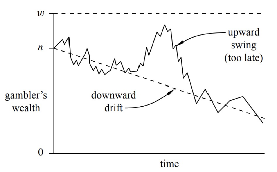
Our intuition is that if the gambler starts with, say, a billion dollars, then he is sure to play for a very long time, so at some point there should be a lucky, upward swing that puts him $100 ahead. But his capital is steadily drifting downward. If the gambler does not have a lucky, upward swing early on, then he is doomed. After his capital drifts downward by tens and then hundreds of dollars, the size of the upward swing the gambler needs to win grows larger and larger. And as the size of the required swing grows, the odds that it occurs decrease exponentially. As a rule of thumb, drift dominates swings in the long term.

We can quantify these drifts and swings. After \(k\) rounds for \(k \leq \text{min}(m, n)\), the number of wins by our player has a binomial distribution with parameters \(p < 1/2\) and \(k\). His expected win on any single bet is \(p - q = 2p - 1\) dollars, so his expected capital is \(n - k (1 - 2p)\). Now to be a winner, his actual number of wins must exceed the expected number by \(m + k (1 - 2p)\). But from p the formula (19.3.10), the binomial distribution has a standard deviation of only \(\sqrt{kp(1-p)}\). So for the gambler to win, he needs his number of wins to deviate by

\[\nonumber \frac{m + k(1 - 2p)}{\sqrt{kp(1-2p)}} = \Theta(\sqrt{k})\]

times its standard deviation. In our study of binomial tails, we saw that this was extremely unlikely.

In a fair game, there is no drift; swings are the only effect. In the absence of downward drift, our earlier intuition is correct. If the gambler starts with a trillion dollars then almost certainly there will eventually be a lucky swing that puts him $100 ahead.

How Long a Walk?

Now that we know the probability, \(w_n\), that the gambler is a winner in both fair and unfair games, we consider how many bets he needs on average to either win or go broke. A linear recurrence approach works here as well.

For fixed \(p\) and \(T\), let \(e_n\) be the expected number of bets until the game ends when the gambler’s initial capital is \(n\) dollars. Since the game is over in zero steps if \(n = 0\) or \(T\), the boundary conditions this time are \(e_0 = e_T = 0\).

Otherwise, the gambler starts with \(n\) dollars, where \(0 < n < T\). Now by the conditional expectation rule, the expected number of steps can be broken down into the expected number of steps given the outcome of the first bet weighted by the probability of that outcome. But after the gambler wins the first bet, his capital is \(n + 1\), so he can expect to make another \(e_{n+1}\) bets. That is,

\[\nonumber \text{Ex}[e_n \mid \text{gambler wins first bet}] = 1 + e_{n+1}.\]

Similarly, after the gambler loses his first bet, he can expect to make another en1 bets:

\[\nonumber \text{Ex}[e_n \mid \text{gambler loses first bet}] = 1 + e_{n-1}.\]

So we have

\[\begin{aligned} e_n &= p \text{Ex}[e_n \mid \text{gambler wins first bet}] + q \text{Ex}[e_n \mid \text{gambler loses first bet}] \\ &= p(1 + e_{n+1}) + q(1 + e_{n-1}) = pe_{n+1} + qe_{n-1} + 1. \end{aligned}\]

This yields the linear recurrence

\[\label{20.1.10} e_{n+1} =\frac{1}{p} e_n - \frac{q}{p} e_{n-1} - \frac{1}{p}.\]

The routine solution of this linear recurrence yields:

Theorem \(\PageIndex{3}\)

In the Gambler’s Ruin game with initial capital \(n\), target \(T\), and probability \(p\) of winning 8 each bet,

\[\label{20.1.11} \text{Ex}[\textit{number of bets}]=\left\{\begin{array}{ll}n(T - n)& \textit{ for } p = \dfrac{1}{2}, \\ \dfrac{w_n \cdot T - n}{p - q} & \textit{ for } p \neq \dfrac{1}{2} \textit{ where } w_n = (r^n - 1) / (r^T - 1) = \text{Pr}[\textit{the gambler wins}]. \end{array}\right.\]

In the unbiased case, (\ref{20.1.11}) can be rephrased simply as

\[\label{20.1.12} \text{Ex}[\text{number of fair bets}] = \text{initial capital } \cdot \text{ intended profit}\]

For example, if the gambler starts with $10 dollars and plays until he is broke or ahead $10, then \(10 \cdot 10 = 100\) bets are required on average. If he starts with $500 and plays until he is broke or ahead $100, then the expected number of bets until the game is over is \(500 \times 100 = 50,000\). This simple formula (\ref{20.1.12}) cries out for an intuitive proof, but we have not found one (where are you, Pascal?).

Quit While You Are Ahead

Suppose that the gambler never quits while he is ahead. That is, he starts with \(n>0\) dollars, ignores any target \(T\), but plays until he is flat broke. Call this the unbounded Gambler’s ruin game. It turns out that if the game is not favorable, that is, \(p \leq 1/2\), the gambler is sure to go broke. In particular, this holds in an unbiased game with \(p = 1/2\).

Lemma 20.1.4. If the gambler starts with one or more dollars and plays a fair unbounded game, then he will go broke with probability 1.

Proof. If the gambler has initial capital \(n\) and goes broke in a game without reaching a target \(T\), then he would also go broke if he were playing and ignored the target. So the probability that he will lose if he keeps playing without stopping at any target \(T\) must be at least as large as the probability that he loses when he has a target \(T > n\).

But we know that in a fair game, the probability that he loses is \(1 - n/T\). This number can be made arbitrarily close to 1 by choosing a sufficiently large value of \(T\). Hence, the probability of his losing while playing without any target has a lower bound arbitrarily close to 1, which means it must in fact be 1. \(\quad \blacksquare\)

So even if the gambler starts with a million dollars and plays a perfectly fair game, he will eventually lose it all with probability 1. But there is good news: if the game is fair, he can “expect” to play forever:

Lemma 20.1.5. If the gambler starts with one or more dollars and plays a fair unbounded game, then his expected number of plays is infinite.

A proof appears in Problem 20.2.

So even starting with just one dollar, the expected number of plays before going broke is infinite! This sounds reassuring—you can go about your business without worrying about being doomed, because doom will be infinitely delayed. To illustrate a situation where you really needn’t worry, think about mean time to failure with a really tiny probability of failure in any given second—say \(10^{-100}\). In this case you are unlikely to fail any time much sooner than many lifetimes of the estimated age of the universe, even though you will eventually fail with probability one.

But in general, you shouldn’t feel reassured by an infinite expected time to go broke. For example, think about a variant Gambler’s Ruin game which works as follows: run one second of the process that has a \(10^{-100}\) of failing in any second. If it does not fail, then you go broke immediately. Otherwise, you play a fair, unbounded Gambler’s Ruin game. Now there is an overwhelming probability, \(1 - 10^{-100}\), that you will go broke immediately. But there is a \(10^{-100}\) probability that you will wind up playing fair Gambler’s Ruin, so your overall expected time will be at least \(10^{-100}\) times the expectation of fair Gambler’s Ruin, namely, it will still be infinite.

For the actual fair, unbounded Gambler’s Ruin gain starting with one dollar, there is a a 50% chance the Gambler will go broke after the first bet, and a more than \(15/16\) chance of going broke within five bets, for example. So infinite expected time is not much consolation to a Gambler who goes broke quickly with high probability.

¹Here we’re legitimately appealing to infinite linearity, since the payoff amounts remain bounded independent of the number of bets.