
3.14: Designing Transfer Functions
- Page ID
- 1755

- This module summarizes the key concepts of transfer functions and includes examples of using transfer functions.
If the source consists of two (or more) signals, we know from linear system theory that the output voltage equals the sum of the outputs produced by each signal alone. In short, linear circuits are a special case of linear systems, and therefore superposition applies. In particular, suppose these component signals are complex exponentials, each of which has a frequency different from the others. The transfer function portrays how the circuit affects the amplitude and phase of each component, allowing us to understand how the circuit works on a complicated signal. Those components having a frequency less than the cutoff frequency pass through the circuit with little modification while those having higher frequencies are suppressed. The circuit is said to act as a filter, filtering the source signal based on the frequency of each component complex exponential. Because low frequencies pass through the filter, we call it a lowpass filter to express more precisely its function.
We have also found the ease of calculating the output for sinusoidal inputs through the use of the transfer function. Once we find the transfer function, we can write the output directly as indicated by the output of a circuit for a sinusoidal input.
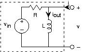
Let's apply these results to a final example, in which the input is a voltage source and the output is the inductor current. The source voltage equals:
\[V_{in}=2\cos (2\pi 60t)+3 \nonumber \]
We want the circuit to pass constant (offset) voltage essentially unaltered (save for the fact that the output is a current rather than a voltage) and remove the 60 Hz term. Because the input is the sum of two sinusoids--a constant is a zero-frequency cosine--our approach is
- find the transfer function using impedances
- use it to find the output due to each input component
- add the results
- find element values that accomplish our design criteria
Because the circuit is a series combination of elements, let's use voltage divider to find the transfer function between Vin and V, then use the v-i relation of the inductor to find its current.
\[\frac{I_{out}}{V_{in}}=\frac{i2\pi fL}{R+i2\pi fL}\frac{1}{i2\pi fL} \nonumber \]
\[\frac{I_{out}}{V_{in}}=\frac{1}{i2\pi fL+R} \nonumber \]
\[\frac{I_{out}}{V_{in}}=H(f) \nonumber \]
where voltage divider
\[voltage\; \; divider=\frac{i2\pi fL}{R+i2\pi fL} \nonumber \]
\[inductor\; \; admittance=\frac{1}{i2\pi fL} \nonumber \]
[Do the units check?] The form of this transfer function should be familiar; it is a lowpass filter, and it will perform our desired function once we choose element values properly.
The constant term is easiest to handle. The output is given by:
\[3\left | H(0) \right |=\frac{3}{R} \nonumber \]
Thus, the value we choose for the resistance will determine the scaling factor of how voltage is converted into current. For the 60 Hz component signal, the output current is
\[2\left | H(60) \right |\cos \left ( 2\pi 60t+\angle (H(60)) \right ) \nonumber \]
The total output due to our source is:
\[i_{out}=2\left | H(60) \right |\cos \left ( 2\pi 60t+\angle (H(60)) \right )+3\times H(0) \nonumber \]
The cutoff frequency for this filter occurs when the real and imaginary parts of the transfer function's denominator equal each other. Thus,
\[2\pi f_{c}L=R \nonumber \]
\[f_{c}=\frac{R}{2\pi L} \nonumber \]
We want this cutoff frequency to be much less than 60 Hz. Suppose we place it at, say, 10 Hz. This specification would require the component values to be related by
\[\frac{R}{L}=20\pi =62.8 \nonumber \]
The transfer function at 60 Hz would be
\[\left | \frac{1}{i2\pi 60L+R} \right |=\frac{1}{R}\left | \frac{1}{6i+1} \right |=\frac{1}{R}\frac{1}{\sqrt{37}}\simeq 0.16\times \frac{1}{R} \nonumber \]
which yields an attenuation (relative to the gain at zero frequency) of about 1/6, and result in an output amplitude of 0.3/R relative to the constant term's amplitude of 3/R. A factor of 10 relative size between the two components seems reasonable. Having a 100 mH inductor would require a 6.28 Ω resistor. An easily available resistor value is 6.8 Ω; thus, this choice results in cheaply and easily purchased parts. To make the resistance bigger would require a proportionally larger inductor. Unfortunately, even a 1 H inductor is physically large; consequently low cutoff frequencies require small-valued resistors and large-valued inductors. The choice made here represents only one compromise.
The phase of the 60 Hz component will very nearly be -π/2 leaving it to be:
\[\frac{0.3}{R}\cos \left ( 2\pi 60t-\frac{\pi }{2} \right )=\frac{0.3}{R}\sin (2\pi 60t) \nonumber \]
The waveforms for the input and output are shown below:
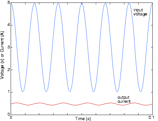
Note that the sinusoid's phase has indeed shifted; the lowpass filter not only reduced the 60 Hz signal's amplitude, but also shifted its phase by 90°.