5.6: Unipolar Space Charge Dynamics - Self-Precipitation

Complementary assumptions in Secs. 5.3 -5.5 are that the effect of the electric field on the flow can be ignored, and that the volume space charge density makes a negligible contribution to the imposed field. Although often good approximations in predicting the trajectories of dilute ions and charged macroscopic particles in moving gases and liquids, these are usually not good assumptions if there is to be an appreciable coupling between the electric field and the neutral fluid through which the charged particles migrate.

What are the effects of "self-fields" (space-charge contributions) left out in the imposed field approximation used in Secs 5.3 -5.5? In this and the next section, this question is addressed while again considering a single species of either positively or negatively charged particles.The pertinent laws are Eqs. 5.2.9 -5.2.11 without source or recombination contributions \((G-R=0)\) and with lengths of interest large enough to justify ignoring diffusion. In writing Eq. 5.2.9, the creation of a field divergence by the space charge is recognized by substituting on the right with Gauss' law, Eq. 5.2.10:

\[ \frac{\partial{\rho_{\pm}}}{\partial{t}} + (\overrightarrow{v} \pm b_{\pm} \overrightarrow{E}) \cdot \nabla \rho_{\pm} = - \frac{\rho_{\pm}^2 b_{\pm}}{\varepsilon}\label{1} \]

This expression is converted to one describing how the charge density changes with time for an observer moving along a characteristic (or force) line by following the procedure developed in Sec. 5.3.2. In-stead of Eq. 5.3.3, Equation \ref{1} becomes

\[ \frac{d \rho_{\pm}}{dt} = - \frac{\rho_{\pm}^2 b_{\pm}}{\varepsilon} \label{2} \]

along the characteristic lines

\[ \frac{d \overrightarrow{r}}{dt} = \overrightarrow{v} \pm b_{\pm} \overrightarrow{E} \label{3} \]

Although the velocity \(\overrightarrow{v}\) is still considered to be imposed, \(\overrightarrow{E}\) in Equation \ref{3} has contributions from not only charges on the boundaries, but from those within the volume of interest as well. So it is that the time dependence of the charge density can be determined from an integration of Equation \ref{2}. For a characteristic line originating when \(t = 0\) where \(\rho_{\pm} = \rho_o\)

\[ \int_{\rho_o}^{\rho_{\pm}} \frac{d \rho_{\pm}}{\rho_{\pm}^2} = - \frac{b_{\pm}}{\varepsilon} \int_o^t dt \label{4} \]

Thus,

\[ \frac{\rho_{\pm}}{\rho_o} = \frac{1}{1 + t/ \tau_e}; \, \tau_e = \frac{\varepsilon}{\rho_o b_{\pm}} \label{5} \]

This result is both remarkably general and somewhat deceiving. Without apparent regard for the particulars of a physical situation, for the boundary conditions and hence for any imposed component of the field and for the locations of charges that image those evolving in the volume, the decay law of Equation \ref{5} is deduced. But, the law applies for an observer measuring time as he follows a given particle along a characteristic line, defined by Equation \ref{3}, originating when \(t = 0\) where \(\rho_{\pm} = \rho_o\). At each step in the evolution, all of the charge (in the volume and on the boundaries) instantaneously contributes to \(\overrightarrow{E}\).This contribution is embodied in Gauss' law. The characteristic viewpoint is now used to make some general deductions, and then by way of illustration, to make specific predictions.

General Properties

Suppose that when \(t=0\) the charged particles are uniformly distributed over some confined region \(V\) within the total volume, as suggested by Fig. 5.6.1. When \(t = 0\), the volume of interest consists of regions either occupied by no charge density or by the uniform density \(\rho_u\). At a later time, the cloud of charged particles has changed its shape and general location. Particles initially at the locations \(A, B\) and \(C\) are respectively found at \(A', B'\) and \(C'\). At a point like \(A'\), with a characteristic line originating within the initial cloud of particles, the charge density is given by Equation \ref{5} as

\[ \rho_{\pm} = \frac{\rho_u}{1 + t/ \tau_e}; \, \tau_e \equiv \frac{\varepsilon}{\rho_u b_{\pm}} \label{6} \]

Note that \(\tau_e\) is itself dependent on the initial charge density.

Now, consider the time dependence of \(\rho_+\) at a fixed location \(A'\). So long as \(A'\) is within the region occupied by the charge cloud, this time dependence is also given by Equation \ref{6}. At each instant, the point in question can be traced backward in time to a location in the cloud when \(t = 0\) where the charge density is the same number, \(\rho_u\). As time progresses, different locations originate the characteristic \(A'\), but because \(\rho_u\) is the same throughout the initial cloud, each of these has the same charge density \(\rho_u\) or no charge density at all. That is, at a position like \(B'\), the characteristic originates on no charge density, and there is no charge density at the instant in question.

Fig. 5. When \(t=0\), charge, having density \(\rho_u\), is uniformly distributed over \(V\). By the time \(t\), it is distributed over \(V'\) with by Equation \ref{6}.

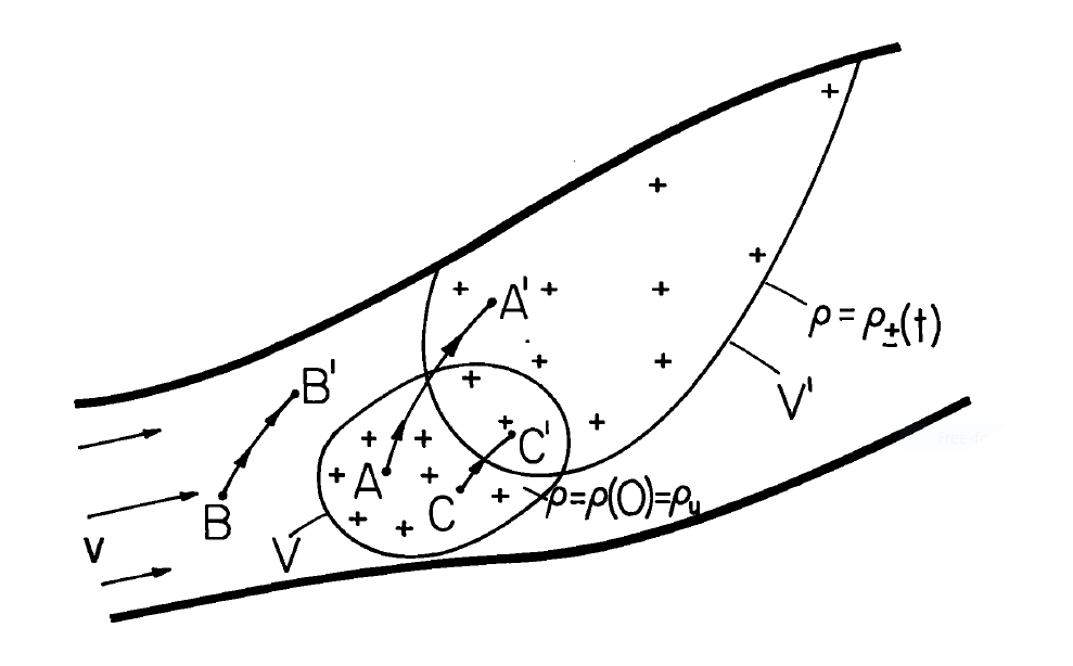
So it is that the charge transient at any fixed location consists of either a charge density decaying according to Equation \ref{6} or no charge density at all. Generally, at a position like \(A'\), the charge density is zero until the "front" arrives. Then, the position \(A'\) is enveloped by the particle cloud which is expanding under its self-field so that the density decays in accordance with Equation \ref{6}. At a position like \(C'\), there is no delay in the arrival of this front so that- the decay is given by Equation \ref{6} from time \(t=0\). But, the time may come when the cloud passes beyond the point in question and the decay in charge density is then abruptly terminated by the density going to zero. When the front arrives and when the cloud has passed by is a matter that must be resolved by integrating to find the characteristic lines.

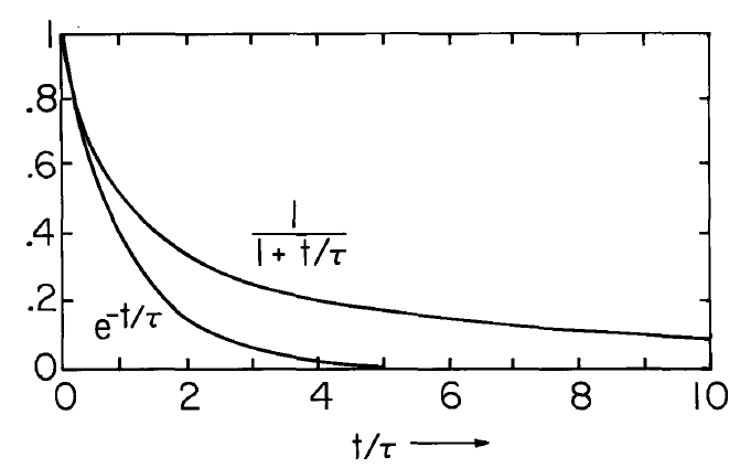
The tendency of the cloud to expand or self precipitate, as the cloud as a whole is carried by the deforming medium and the total field, is described by a decay that is relatively slow. Figure 5.6.2 emphasizes this point by comparing Equation \ref{7} to an exponential decay.

Fig. 5.6.2. Comparison of self-presipitation transient to exponential decay.

The rate of decay along a characteristic line represented by \(\tau_e\) is the same as the charging time constant for the "drop" in Sec. 5.5. An important observation can now be made relevant to taking into account space-charge effects on the collection of charged particles by isolated drops. If space-charge effects are really important, then processes of interest must occur on the time scale of \(\tau_e\). This implies that the drop described in Sec. 5.5 must change its charge in a time on this same scale. But, the drop charge contributes to the electric field, and in the analysis of Sec. 5.5 the electric field is assumed to be constant during the time that a particle migrates several drop radii. Thus it is apparent that if space-charge contributions to the field are to be taken into account, the quasi-steady approximation is not valid.

A Space-Charge Transient

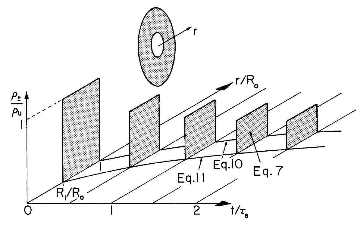
As a simple illustration of the fate of a cloud of charged particles that is initially of uniform charge density, consider the radially symmetric configuration of Fig. 5.6.3. When \(t = 0\), the particles occupy the annular region \(R_i < r < R_o\). Image charges are presumed sufficiently remote that the field can be regarded as radially symmetric. There is a source of fluid inside the region \(r < R_i\) giving rise to a volume rate of flow \(\phi_v\) \((m^3/sec)\). Because the flow is incompressible,the resulting velocity distribution is determined by the requirement that the material flux at any radius \(r\) be the same: \(4 \pi r^2 v_r = \phi_v\). The characteristic lines are then found from the one nontrivial component of Equation \ref{3}:

\[ \frac{dr}{dt} = \frac{\phi_v}{4 \pi r^2} \pm b_{\pm} E_r \label{7} \]

Because the initial charge distribution is uniform, any region within the cloud is known to have a density that decays according to Equation \ref{6}. In this simple example it is easy to find the position of the outward propagating front, and hence locate the region where this decay applies. By the integral form of Gauss' law, Eq. 2.7.1a, the electric field at \(r\), the leading edge of the cloud, is

\[ E_r = \pm \frac{1}{3} \frac{(R_o^3 - R_i^3) \rho_u}{\varepsilon r^2} \label{8} \]

Substitution of this expression into Equation \ref{7} and integration gives

\[ \frac{r}{R_o} = \Big \{1 + \big[ \frac{3 \phi_v \tau_e}{4 \pi R_o^3} + 1 - (\frac{R_i}{R_o})^3 \big] \frac{t}{\tau_e} \Big \}^{1/3} \label{9} \]

Similar arguments apply to the trailing edge, where \(E_r =0\) and hence

\[ \frac{r}{R_o} = \Big [ \big ( \frac{R_i}{R_o} \big )^3 + \big ( \frac{3 \phi_v \tau_e}{4 \pi R_o^3} \big ) \frac{t}{\tau_e} \Big ] ^{1/3} \label{10} \]

These last two expressions define the region occupied by the charged particles. During the time that the particles surround a given fixed radial location, the temporal decay at that radius is given by Equation \ref{6}. The evolution of the cloud is illustrated in Fig. 5.6.3. Fig.

Fig. 5.6.3. When \(t = 0\), a uniform density \(\rho_u\) of charged particles fills the spherical shell \(R_i < r < R_o\). A source of gas at the origin imparts a radial velocity. For this plot, \(R_o/R_i = 0.5, \, 3 \phi_v \tau_e/4 R_o^3 = 1\). Remember that the charge is self-precipitating in three dimensions. At any time, the product of the charge density and the volume of the region filled by the charge is constant.

Steady-State Space-Charge Precipitator

What from the laboratory frame of reference appears to be steady or stationary phenomenon is from the particle frame of reference still a transient. The characteristic time is typically a transport time \(l/U\), and the ratio

\[ R_e = \frac{\tau_e}{l/U} = \frac{U \varepsilon_o}{l \rho_o b_{\pm}} \label{11} \]

represents the degree to which convection competes with self-field migration in determining the distribution of the charged particles. \(R_e\) is defined as the electric Reynolds number.

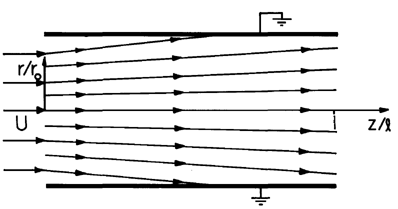
As a specific illustration, consider the circular cylindrical duct shown in Fig. 5.6.4. Gas enters at the left with a uniform velocity profile carrying a uniform distribution of charged particles. The channel wall is at zero potential, and hence only the self-fields contribute to the migration. With the assumption that variations in the \(z\) direction of the particle density occur relatively slowly goes the quasi-one-dimensional model of an electric field that is dominantly in the radial direction. Hence, the characteristic lines are determined from Equation \ref{3} approximated as

\[ \frac{d \overrightarrow{r}}{dt} = U \overrightarrow{i}_z \pm b_{\pm} E_r(r) \overrightarrow{i}_r \label{12} \]

The \(z\) component of this expression can be integrated to describe the characteristic line associated with the solution given by Equation \ref{6}, i.e., for the particles entering at \(z = 0\), where \(\rho_+ = \rho_o = \rho_u\) when \(t = 0\):

\[ z = Ut \label{13} \]

Hence, the distribution of charge density with \(z\) is obtained directly by substituting Equation \ref{13} into Equation \ref{6}.

\[ \rho_{\pm} = \frac{\rho_u}{1 + \frac{z}{l} (\frac{l}{U \tau_e})} \label{14} \]

Fig. 5.6.4 Space-charge precipitator having circular cylindrical cross section and \(R_e = 1\) showing characteristic lines.

The fact that the axial component of \(\overrightarrow{E}\) is neglected has made it possible to find the spatial distribution of \(\rho_{\pm}\) without solving the self-consistent characteristic equations.

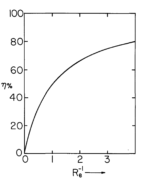
A length \(l\) of the channel might be used as a precipitator, for the removal of pollutant particles which are charged upstream. The cleaning efficiency of such a device follows from Equation \ref{14} integrated over the channel cross section \(A\) at \(z = l\) and \(z = 0\),

\[ \mu \equiv \frac{ \int_A \rho_u da - \int_A \rho+{\pm} (l) da }{\int_A \rho_u da} = \frac{R_e^{-1}}{1 + R_e^{-1} } \label{15} \]

and is determined by the ratio of transport time to \(\tau_e\).The dependence of \(\mu\) on \(R_e\) is shown in Fig. 5.6.5. The relatively poor efficiency even with a residence time several times \(\tau_e\) has its origins in the relatively slow decay depicted Fig. 5.6.2.

The trajectories of the particles are determined from both the radial and axial components of Equation \ref{12}. Gauss' law relates the charge density at a given cross section along the \(z\) axis to \(E_r\) :

\[ \frac{1}{r} \frac{\partial}{\partial{r}} (r E_r) = \pm \frac{\rho_{\pm}}{\varepsilon_o} \label{16} \]

Fig. 5.6.5. Efficiency of space-charge precipitator as function of reciprocal electric Reynolds number, the ratio of residence time to \(\tau_e\).

This expression can be integrated in the radial direction to give

\[ E_r = \pm \frac{1}{r} \int_o^r \frac{r}{\varepsilon_o} \frac{\rho_u dr}{(1 + \frac{z}{l} R_e^{-1})} = \pm \frac{1}{2} \frac{r}{\varepsilon_o} \frac{\rho_u}{(1 + \frac{z}{l} R_e^-1)} \label{17} \]

Thus, the radial component of Equation \ref{12} becomes

\[ \frac{dr}{dt} = \frac{1}{2} b_{\pm} \frac{r}{\varepsilon_o} \frac{\rho_u}{1 + \frac{z}{l} R_e^-1} \label{18} \]

But, in view of the axial component of this same equation,

\[ \frac{dr}{dt} = \frac{dr}{dz} \frac{dz}{dt} = U \frac{dr}{dz} \label{19} \]

Thus, the time is eliminated as a parameter to obtain an equation for the characteristic line in the \((r,z)\) plane. Integration of Eqs. \ref{18} and \ref{19} gives

\[ \frac{r}{r_o} = \sqrt{1 + \frac{z}{l} R_e^{-1}} \label{20} \]

Which trajectory is considered is determined by \(r_o\), the radial position at which a particle enters where \(z = 0\). A sketch of the characteristic lines is included with Fig. 5.6.4.