5.9: Conductivity and Net Charge Evolution with Generation and Recombination- Ohmic Limit
- Page ID
- 51053
The net free charge density and conductivity for the bipolar systems treated in Sec. 5.8, defined as
\[ \rho_f \rho_+ - \rho_{-}; \, \sigma = b_+ \rho_+ + b_{-} \rho_{-} \label{1} \]
are natural variables for understanding the relationship between charge migration and relaxation. In terms of \((\rho_f,\sigma)\), the charge densities \(\rho_+\) and \(\rho_{-}\). are found by inverting Eqs. \ref{1}:
\[ \rho_{\pm} = \frac{\sigma \pm b_{\pm} \rho_f}{b_+ + b_{-}} \label{2} \]
With the objective of casting the charge evolution in terms of pf and a, the difference is taken between the conservation equations for \(+\) and \(-\) species, Eqs. 5.8.9, and \(\rho_+\) and \(\rho_{-}\) are replaced on the right using Eqs. \ref{2}:
\[ \frac{D \rho_f}{Dt} = - \overrightarrow{E} \cdot \nabla \sigma - \frac{\sigma \rho_f}{\varepsilon} + \Big (\frac{K_+ - K_{-}}{b_+ - b_{-}} \Big ) \nabla^2 \sigma + \Big (\frac{K_+ b_{-} - K_{-} b_+}{b_+ - b_{-}} \Big ) \nabla^2 \rho_f \label{3} \]
To similarly obtain an expression for a, Eqs. 5.8.9 are respectively multiplied by b+ and summed to obtain
\[ \frac{D \sigma}{D t} = - \overrightarrow{E} \cdot \nabla [ (b_+ - b_{-}) \sigma + b_+ b_{-} \rho_f] - [ (b_+ - b_{-}) \sigma + b_+ b_{-} \rho_f] \frac{\rho_f} {\varepsilon} + (b_+ - b_{-}) \beta n \\ - \frac{\alpha}{q (b_+ + b_{-})} [ \sigma^2 - (b_+ - b_{-}) \sigma \rho_f - b_+ b_{-} \rho_f^2] + \Big (\frac{K_+ b_{+} - K_{-} b_{-}}{b_+ - b_{-}} \Big ) \nabla^2 \sigma + \frac{b_+ b_{-}}{b_+ + b_{-}} (K_+ - K_{-}) \nabla^2 \rho_f \label{4} \]
To complete the description, Eqs. \ref{2} are used to write Eq. \ref{10} as
\[ \frac{Dn}{Dt} = \frac{-\beta}{q} n + \frac{\alpha}{q^2 (b_+ + b_{-})^2} [ \sigma^2 - (b_+ - b_{-}) \sigma \rho_f - b_{+} b_{-} \rho_f^2] + K_D \nabla^2 n \label{5} \]
These last three expressions are an alternative to Eqs. 5.8.9 and 5.8.10 in describing the migration and diffusion of the carriers in a deforming material. The method of characteristics could be used to solve these expressions, much as illustrated in Sec. 5.8. But the objective in this section is to identify the rate processes encapsulated by these laws and hence to discern the dominant contributions to the equations. Limiting forms of the equations, for example the ohmic model emphasize here and used in the remainder of this chapter, are necessary if the conduction laws are to be embodied in models that bring in still other dynamical processes.
The approach now used is similar to that introduced in Sec. 2.3, where the quasistatic limits of the electrodynamic laws are recognized by using a normalization of the laws to discern the critical characteristic times. Given that dynamical times of interest are characterized by \(\tau\), what are the times characterizing the processes represented by Eqs. \ref{3} - \ref{5}?
Variables are normalized such that
\[ t = \underline{t} \tau, \, (x,y,z) = (\underline{x},\underline{y},\underline{z})l, \, \overrightarrow{v} = \underline{\overrightarrow{v}}l/ \tau, \, \sigma = \underline{\sigma} \Sigma, \, \overrightarrow{E} = \underline{\overrightarrow{E}} \mathscr{E}, \, \underline{\rho_f} = \underline{\rho_f} \varepsilon \mathscr{E}/l \label{6} \]
Thus, \(\Sigma\) is a typical electrical conductivity and \(\mathscr{E}\) is a typical electric field intensity. The free charge density is normalized so that it is typically the charge density that would "shield out" the field \(\mathscr{E}\) in the distance \(l\). In the state of equilibrium where the charge density is zero, while \(\sigma\) and \(n\) are uniform and constant, the generation and recombination terms balance. Thus, at each point
\[ \frac{\beta}{q} = \frac{\alpha \sigma^2}{q^2 (b_+ + b_{-})^2 n} \label{7} \]
This expression makes it possible to use equilibrium data to evaluate the generation coefficient, given the parameters on the right. It also suggests that the neutral number density be normalized such that
\[ n = \underline{n} \frac{\alpha \Sigma^2}{q (b_+ + b_{-})^2 \beta} \label{8} \]
Introduction of these normalizations into Eqs. \ref{3} - \ref{5} results in the expressions
\[ \frac{D \rho_f}{Dt} = \frac{\tau}{\tau_e} (- \overrightarrow{E} \cdot \nabla \sigma - \sigma \rho_f) + \frac{\tau}{\tau_e} \frac{\tau_{mig}}{\tau_D} \frac{(K_+ - K_{-})(b_+ + b_{-})}{K_+ b_{-} + K_{-} b_{+})} \nabla^2 \sigma + \frac{\tau}{\tau_D} \nabla^2 \rho_f \label{9} \]
\[ \frac{D \sigma}{D t} = - \frac{\tau}{\tau_{mig}} \frac{(b_+ - b_{-})}{(b_+ + b_{-})} (\overrightarrow{E} \cdot \nabla \sigma + \sigma \rho_f) - \frac{\tau}{\tau_{mig}} \frac{\tau_e}{\tau_{mig}} \frac{b_+ b_{-}}{(b_+ + b_{-})^2} (\overrightarrow{E} \cdot \nabla \rho_f + \rho_f^2) \\ + \frac{\tau}{\tau_e} [ \frac{\varepsilon \alpha}{(b_+ + b_{-}) q}]n - \frac{\tau}{\tau_e} [ \frac{\varepsilon \alpha}{(b_+ + b_{-}) q}] \sigma^2 + \frac{\tau}{\tau_{mig}} [ \frac{\varepsilon \alpha}{(b_+ + b_{-}) q}] \Big (\frac{b_+ - b_{-}}{b_+ + b_{-}} \Big ) \sigma \rho_f \\ + \frac{\tau}{\tau_{mig}} \frac{\tau_e}{\tau_{mig}} [ \frac{\varepsilon \alpha}{(b_+ + b_{-}) q}] \frac{b_+ b_{-}}{(b_+ + b_{-})^2} \rho_f^2 + \frac{(K_+ b_+ + K_{-} b_{-})}{(K_+ b_{-} + K_{-} b_+)} \nabla^2 \sigma \\ + \frac{\tau}{\tau_{mig}} \frac{\tau_e}{\tau_D} \frac{b_+ b_{-}}{(b_+ + b_{-})^2} \frac{(K_+ - K_{-})(b_+ + b_{-})}{(K_+ b_{-} + K_{-} b_{+})} \nabla^2 \rho_f \label{10} \]
\[ \frac{D_n}{D_t} = - \frac{\tau}{\tau_{th}} n + \frac{\tau}{\tau_{th}} [ \underline{\sigma}^2 - \frac{(b_+ - b_{-})}{(b_+ + b_{-})} \frac{\tau_e}{\tau_{mig}} \sigma \rho_f - \frac{b_+ b_{-}}{(b_+ + b_{-})^2} \Big ( \frac{\tau_e}{\tau_{mig}} \Big ) ^2 \rho_f^2] + \frac{\tau}{\tau_D} \frac{K_D (b_+ + b_{-})}{(K_+ b_{-} + K_{-} b_{+})} \nabla^2 n \label{11} \]
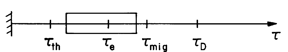
where the following characteristic times have been identified
\[ \tau_e \equiv \frac{\varepsilon}{\Sigma}, \, \tau_{mig} \equiv \frac{1}{\mathscr{E} (b_+ + b_{-})}, \, \tau_D \equiv \frac{l^2}{[\frac{K_+ b_{-} + K_{-} b_+}{b_+ + b_{-}}]}, \, \tau_{th} = \frac{q}{\beta} \label{12} \]
The other dimensionless coefficients in Eqs. \ref{9} - \ref{11} are typically of the order of unity. (Note that at least for Langevin recombination, where \(\alpha\) is given by Eq. 5.8.4, the coefficient \(\varepsilon \alpha/ (b_+ + b_{-}) q\) is unity).
With the objective of ordering the time constants of Eq. \ref{13}, \(\tau_{th}\) is estimated by substituting the equilibrium values given by Eq. \ref{7}, \(\alpha\) from Eq. 5.8.4 and \(\sigma = (n_+ b_+ + n_{-} b_{-}) q\):
\[ \tau_{th} \equiv \frac{q}{\beta} \se \frac{q^2 (b_+ + b_{-})^2n}{\alpha \sigma^2} = \tau_e \frac{n}{(n_+ b_+ + b_{-} b_{-})/(b_+ + b_{-})} \label{13} \]
Thus, \(\tau_{th}\) is essentially \(\tau_e\) multiplied by the ratio of the neutral to the charged particles. If \(\beta\) is large enough that essentially all of the particles available are ionized, then \(\tau_{th}\) is a small fraction of the charge relaxation time \(\tau_e\).
The ordering of characteristic times shown in Fig. 5.9.1 is typical if a configuration is to be appropriately modeled as "ohmic." Because lengths of interest are relatively large, the diffusion time is extremely long. That the migration time \(\tau_{mig}\) is also long compared to times of interest is also a matter of the length scale of interest, and is justified if the typical electric field intensities are not too large. Times of interest in the ohmic model are arbitrary relative to \(\tau_e\). They can be long or short compared to the charge relaxation time.
With the understanding that the equations are valid for processes in this dynamic range, Eqs. \ref{9} - \ref{11} are approximated by
\[ \frac{D \rho_f}{Dt} = \frac{\tau}{\tau_e} ( - \overrightarrow{E} \cdot \nabla \sigma - \rho_f \sigma) \label{14} \]
\[ \frac{D \sigma}{Dt} = \frac{\tau}{\tau_e} [ \frac{\varepsilon \alpha}{(b_+ + b_{-}) q} ] (n - \sigma^2) \label{15} \]
\[ \frac{Dn}{Dt} = - \frac{\tau}{\tau_{th}} (n - \sigma^2) \label{16} \]
By multiplying Eq. \ref{16} by \((\tau_{th}/\tau_e)[\varepsilon \alpha/(b_+ + b_{-})q]\) and adding it to Eq. \ref{15}, it follows that
\[ \frac{D}{Dt} [ \sigma + \frac{\tau_{th}}{\tau_e} \frac{\varepsilon \alpha}{(b_+ + b_{-})q} n ] = 0 \label{17} \]
Now, if \(\tau_{th}\) is short compared to times of interest, as depicted by Fig. 5.9.1, this expression becomes (with variables written in dimensional form),
\[ \frac{D \sigma}{D t} = 0 \label{18} \]
For an observer attached to a given particle of the material, the conductivity is constant. In this limit, the conductivity can be regarded as a property of the material.
In unnormalized form, Eq. \ref{14} is
\[ \frac{D \rho_f}{D t} = - \frac{\rho_f}{(\varepsilon / \sigma)} - \overrightarrow{E} \cdot \nabla \sigma \label{19} \]
In this charge relaxation expression, \(\alpha\) can now be regarded as a given parameter. These last two expressions constitute the "ohmic" model.
Maxwell's Capacitor
In terms of an ohmic model, the bipolar migration with generation and re-combination is the two-region lossy capacitor of Fig. 5.9.2. The lower region is a fixed material,which according to Eq. \ref{18} conserves its initially uniform conductivity. The upper region is of the same permittivity, but is insulating.
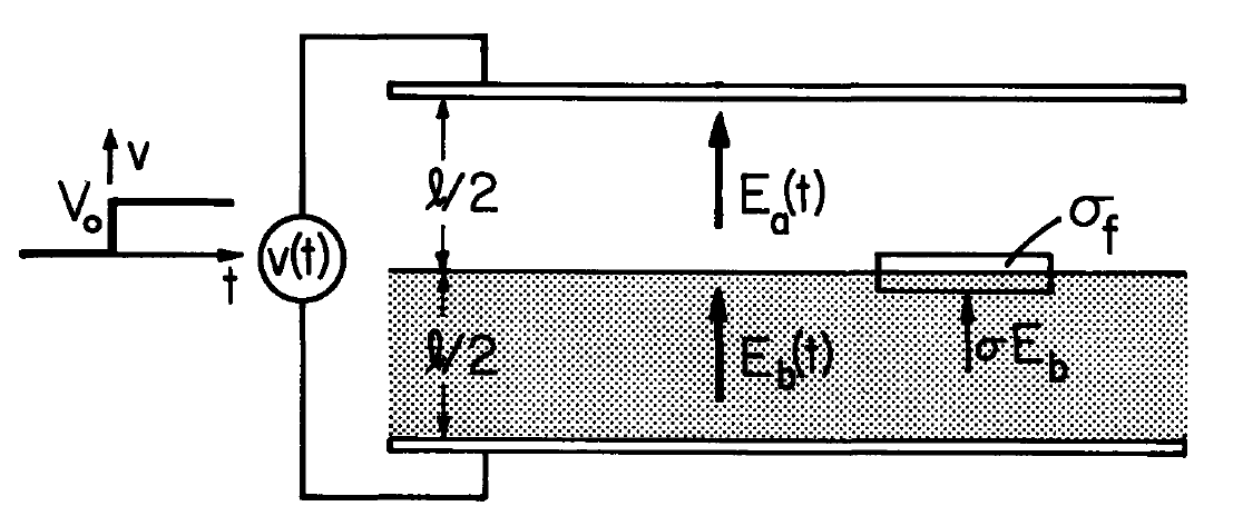
As will be shown in the next section, with the application of a constant voltage \(V_o\) to the electrodes, there is never a net free charge density in the material. Hence, fields in each region are uniform, \(E_a(t)\) and \(E_b(t)\). Because of the voltage constraint,
\[ E_a \frac{l}{2} + E_b \frac{l}{2} = v \label{20} \]
Accumulation of surface charge \(\sigma_f = \varepsilon E_a - \varepsilon E_b\), at the interface between the lossy material and the insulating upper region is caused by the conduction current \(\sigma E_b\) feeding the interface. (This boundary condition is considered in general terms in Sec. 5.11). Thus,
\[ \frac{d}{dt} ( \varepsilon E_a - \varepsilon E_b) = \sigma E_b \label{21} \]
These two expressions combine to give a differential equation for the field inside the lossy material with the applied voltage as a drive:
\[ \frac{dE_b}{dt} + \frac{\sigma}{2 \varepsilon} E_b = \frac{1}{l} \frac{dv}{dt}; \, E_a = {2v}{l} - E_b \label{22} \]
It follows that the transient resulting from the application of a step in voltage to the amplitude \(V_o\) is
\[ E_b = \frac{V_o}{l} e^{-t/ \tau_e}; \, \sigma_f = \frac{2 \varepsilon V_o}{l} [ 1 - e^{-t/ \tau_e}]; \tau_e \equiv 2 \varepsilon/ \sigma \label{23} \]
Numerical Example
(The numerical analysis of this section was carried out by R. S. Withers) Now,by comparing the predictions of the ohmic model to the "exact" solution afforded by the numerical scheme described in Sec. 5.8, consider the response of the Maxwell capacitor to a step in applied voltage. The configuration, shown in Fig. 5.8.3, is initially with the lower half of the region between the electrodes uniformly filled with positive and negative charge densities. In this lower region, generation and re-combination are initially in equilibrium, as represented by Eq. \ref{7}. Thus, there is also an initial uniform distribution of n in the lower region.
With parameters arranged so that the characteristic times have the ordering shown in Fig. 5.9.1,the response to a step in applied voltage is displayed by Fig. 5.9.3. As would be expected from the ohmic Maxwell capacitor model, the electric field in the conducting region, shown by Fig. 5.9.3a,decays exponentially with the time constant Te, while the surface charge "density" builds up with a similar time constant (Eqs. \ref{23}).
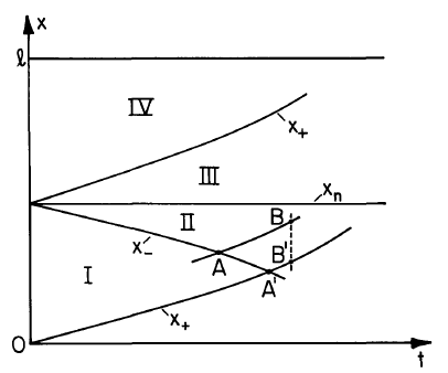
Figure 5.9.4 identifies some of the regions demarked by the three families of characteristics,particularly those emanating from the initial position of the interface. Regions \(I\) and \(IV\) aredescribed by the Maxwell capacitor model. This means that the electric field on the demarking characteristics \(x_+\) and \(x_{-}\). is known. For example, on \(x_{-}\), \(\overrightarrow{E}\) is given by Eq. \ref{23}. Thus, the characteristic equation, Eq. 5.8.15c, can be integrated to delimit region \(I\). In region \(I\), charge neutrality prevails and generation is in equilibrium with recombination.
To further refine the picture, the role of the neutrals in determining the generation of new charged particle pairs must be recognized. Because region \(III\) is "ahead" of the neutral characteristic originating at the interface, this region is one where neutrals can only be created by recombination.
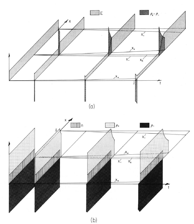
Fig.5.9.3.Evolution of (a) field and free charge density and (b) charged particles and neutrals, with recombination and generation in the Maxwell capacitor configuration of Fig.5.9.2. When \(t=0\), voltage is turned on. Characteristics \(x_+\) and \(x_{-}\) are in the \(x-t\) plane. Neutral characteristics are \(x_n = constant\). For the case shown, \(b_+ = b_{-}\), \(t = t \tau_{mig}\), where \(\tau_{mig}\) is given by Eq.\ref{12} with \(\mathscr{E}=V_o/l\). Also, initially \(\rho_+ = \rho_{-} = 30 \varepsilon_o V_o/l^2\), \(n = \varepsilon_o V_o/q l^2\) (i.e., 30 ion pairs for each neutral so that according to Eq.\ref{13}, \(\tau_{th}=\tau_e/30\) and \(\beta\) is equilibrium value given by Eq.\ref{7}. Recombination is Langevin (Eq.5.8.4).
Because there are no negative charges in this region, there is no recombination and hence no neutrals. Initially, in region \(II\), there are neutrals. However, because of the high degree of ionization intrinsic to the ohmic model (\(tau_{th} << \tau_e)\), the generation in this region (which for lack of negative charges is not balanced by recombination) quickly depletes the neutrals. Essentially, the neutral density in region \(II\) is zero. Thus, in both regions \(II\) and \(III\), essentially unipolar dynamics prevail, with the positive charge density decaying in accordance with Eq. 5.6.6 and the initial charge density, essentially determined by \(\rho_+\) where the characteristic enters region \(II\) from region \(I\), equal to \(\rho_+\) in the equilibrium region.
This unipolar picture of the charge density decay along an x+ characteristic in regions \(II\) and \(III\) explains why \(\rho_+\) decays with increasing \(x\) at any given time. Characteristics \(x_+\) entering region \(II\) at \(A\) and \(A^{'}\) (Fig. 5.9.4) carry the same equilibrium charge density. Thus there is more time for decay of \(\rho_+\) at point \(B\) than there is at \(B^{'}\), even though \(B\) and \(B^{'}\) are at the same instant in time.