
4.3: Classification of Devices and Interactions
- Page ID
- 28140

Based on the developed or linear air-gap configuration of Fig. 4.2.1a, this section begins with illustrative simplified examples of "synchronous" and "d-c" magnetic and electric interactions. Then a general discussion is given of the various classes of machines, some having lumped-parameter models developed in later sections of this chapter and in the problems.
In parallel, consider first the electric and magnetic configurations of Part 1 of Table 4.3.Even though the devices might in fact be developed or "linear," the terms stator and rotor will be used to refer to the elements on respective sides of the air gap. The magnetic field is produced by spatially sinusoidal distributions of current modeled as current sheets on the surfaces of the stator and rotor. Because the stator and rotor are modeled as infinitely permeable, \(\overrightarrow{H} = 0\) outside the air gap and the surface currents "terminate" the tangential fields (Eq. 2.10.21). The electric field is produced by electrodes constrained to have spatially periodic potentials. Thus, boundary conditions at the air-gap boundaries \((s)\) and \((r)\) are
\[ \begin{align} &H_z^s = Re[ \tilde{K}^s \, exp(-jkz)] \quad \quad \quad & \phi^s = Re[ \tilde{V}^s \, exp(-jkz)] \nonumber \\ &H_z^r = Re[ -\tilde{K}^s \, exp(-jkz)] \quad \quad \quad & \phi^r = Re[ \tilde{V}^r \, exp(-jkz)] \nonumber \end{align} \label{1} \]
where \((\tilde{K}^s,\tilde{K}^r)\) and \((\tilde{V}^s,\tilde{V}^r)\) are given complex functions of time. (Complex notation is introduced in Sec. 2.15.)
With the surface \(S_1\) taken as the rotor surface, \((r)\), it follows from Eq. 4.2.1 and the average theorem, Eq. 2.15.14, that the force on a section of the rotor having area \(A\) is
| Sources imposed on moving member | 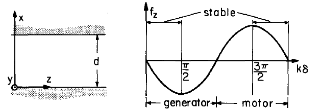 |
|
| 1- Currents (potentials) constrained on both windings (electrodes) | 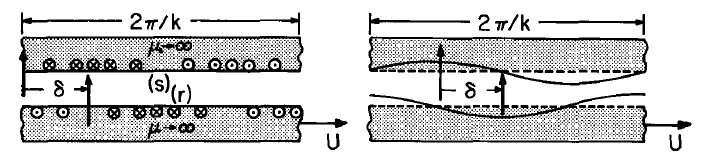 |
|
| 2- Current (potential) constrained on "stator" and permanent magnetization (polarization) on "rotor" | 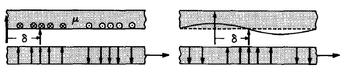 |
|
| 3- Current (potential) constrained on "stator" and flux (charge) constrained on "rotor" | 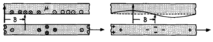 |
|
| Sources instantaneously induced on nonuniform moving member | 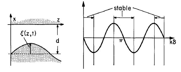 |
|
| 4- Current (potential) constrained on "stator" and magnetization (polarization) induced on "rotor" having saliency | 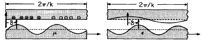 |
|
| 5- Current (potential) constrained on "stator" and current (charges) induced on "rotor" having saliency | 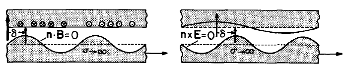 |
|
\[ f_z = \begin{align} &\frac{A}{2} Re \mu_o \, \tilde{H}^r_x (\tilde{H}^r_z)^{*} = \frac{A}{2} Re \mu_o \, \tilde{H}^r_x (-\tilde{K}^r)^{*} \quad \quad \quad &\frac{A}{2} Re \varepsilon_o \, \tilde{E}^r_x (\tilde{E}^r_z)^{*} = \frac{A}{2} Re \varepsilon_o \, \tilde{E}^r_x (jk\tilde{V}^r)^{*} \nonumber \end{align} \label{2} \]
The gap transfer relations, Eq. (a) of Table 2.16.1, give the normal fluxes at \((s)\) and \((r)\) in terms of the potentials there. In the magnetic case, \(H_z= jk\tilde{\psi}\) and because of the boundary conditions, Equation \ref{1}, these relations become
\[\begin{align} &\begin{bmatrix} \mu_o \tilde{H}_x^s \\ \mu_o \tilde{H}_x^r \end{bmatrix} = \mu_o k\begin{bmatrix} -coth \, (kd) & \frac{1}{sinh \, (kd)} \\ -\frac{1}{sinh \, (kd)} & coth \, (kd) \end{bmatrix} \begin{bmatrix} \frac{\tilde{K}^s}{jk} \\ \frac{-\tilde{K}^r}{jk} \end{bmatrix} \nonumber \quad \quad \quad & \begin{bmatrix} \varepsilon_o \tilde{E}_x^s \\ \varepsilon_o \tilde{E}_x^r \end{bmatrix} = \varepsilon_o k\begin{bmatrix} -coth \, (kd) & \frac{1}{sinh \, (kd)} \\ -\frac{1}{sinh \, (kd)} & coth \, (kd) \end{bmatrix} \begin{bmatrix} \tilde{V}^s \\ \tilde{V}^r \end{bmatrix} \nonumber \end{align} \label{3} \]
Substitution of the normal flux densities at \((r)\) expressed by Eqs. \ref{3} into Eqs. \ref{2} gives the desired forces
\[\begin{align} &f_z = -\frac{A \mu_o}{2 sinh \, (kd)} Re [j \tilde{K}^s (\tilde{K}^r)^{*}] \quad \quad \quad &f_z = -\frac{A \varepsilon_o}{2 sinh \, (kd)} Re [j (k\tilde{V}^s) (k\tilde{V}^r)^{*}] \nonumber \end{align} \label{4} \]
Note that the terms involving products of the individual rotor excitations do not contribute. (They are imaginary and hence dropped in taking the real part.) Physically, this is expected because such terms represent the rotor self-field interactions.
Synchronous Interactions: Consider now systems with the rotor excitations produced by windings or electrodes that are fixed to the rotor. The coordinate \(z^{'}\) measures distance from a frame of reference moving with the velocity \(U\) of the rotor, as sketched in Fig. 4.3.1. Fixed and moving frame coordinates are related in the figure. Perhaps through slip rings, the rotor is excited by a current of angular frequency \(\omega_r\), in such way that as viewed from the rotor there is a current or potential distribution taking the form of a traveling wave:

\[ \begin{align} &K^r = K^r_o \, sin[ \omega_r t - k(z^{'} - \delta)] \quad \quad \quad &V^r = -V^r_o \, cos[ \omega_r t - k(z^{'} - \delta)] \nonumber \end{align} \label{5} \]
On the stator, a similar arrangement of windings or electrodes, with excitations at the angular frequency \(\omega_s\), give the traveling waves:
\[ \begin{align} &K^s = K^s_o \, sin[ \omega_s t - kz] \quad \quad \quad &V^s = V^s_o \, cos[ \omega_s t - kz] \nonumber \end{align} \label{6} \]
Because \(z^{'} = z -Ut\), Eqs. \ref{5} and \ref{6} can be written in terms of complex amplitudes:
\[ \begin{align} &\tilde{K}^r = -jK_o^r \, e^{j(\omega_r + kU)t} \, e^{jk \delta} \quad \quad \quad &\tilde{V}^r = -V_o^r \, e^{j(\omega_r + kU)t} \, e^{jk \delta} \nonumber \\ &\tilde{K}^s = -jK_o^s \, e^{j \omega_s t} \quad \quad &\tilde{V}^s = V_o^s \, e^{j \omega_s t} \nonumber \end{align} \label{7} \]
Substitution of these amplitudes into the respective force relations of Equation \ref{4} gives forces with sinusoidal time dependences. The frequencies are in each case \(\omega_s - \omega_r - KU\). Only if this frequency is zero will these forces have time-average values. Division of the resulting frequency condition by \(k\) shows that these time-average forces exist because, as viewed from the stator frame of reference, the velocities of the traveling waves of field induced by stator and rotor sources are equal:
\[ \frac{\omega_s}{k} = \frac{\omega_r}{k} + U \label{8} \]
Usually, the rotor is d-c excited so that \(\omega_r = 0\) and the phase velocity of the stator traveling wave,\(\omega_s/k\), is equal to the rotor velocity \(U\). Under the synchronous condition, the substitution of Eqs. \ref{7} into Eqs. \ref{4} gives the forces as functions of the relative spatial phase \(k \delta\) between traveling waves:
\[ \begin{align} &f_z = -\frac{A \mu_o K_o^s K_o^r}{2 sinh \, kd} sin \, k \delta \quad \quad \quad &f_z = -\frac{A \varepsilon_o (kV_o^s)(kV_o^r)}{2 sinh \, kd} sin \, k \delta \nonumber \end{align} \label{9} \]
The sketches of the stator and rotor excitations in Part 1 of Table 4.3.1 (at the instant \(t = 0\)) show the relative distributions with \(\delta = \lambda/4\), and hence \(k \delta \equiv 2 \pi (\delta/ \lambda) = \pi/2\). According to Eqs. \ref{9}, it is at this spatial phase that the greatest retarding force acts on the rotor. The observation is consistent with what would be expected intuitively for the sketched distributions. Under the synchronous conditions the relative distribution of stator and rotor field sources is invariant. The stator cur-rent distribution gives rise to a normal flux density that peaks at the current null. This is the stator magnetic axis, indicated by the vertical arrow on the stator. This field interacts with the rotor current to produce the time-average force in the -z direction. Stator and rotor magnetic axes tend to line up. Similarly, in regions of positive and negative electrode potential there are positive and negative surface charges (although not exactly in phase with the potential). Thus, the retarding electric force results from the attraction of neighboring opposite charges. The rotor and stator axes,denoted by the vertical arrows, also tend to line up.
The classic force (or torque) phase-angle diagram, the graphical representation of Eqs. \ref{9},is shown at the top of Table 4.3.1. Angles of positive and negative force can respectively give motor and generator operation. But, operation is generally restricted to the shaded regions because then a change in relative phase, \(k \delta\), results in a force that tends to return the rotor to its original angle.
Parts 2 and 3 of Table 4.3.1 illustrate other types of excitations that result in synchronous interactions. In each of these, the rotor sources are "attached" to the rotor and hence the synchronous condition of Equation \ref{8} reduces to \(\omega_s/k = U\). Each has a force with the same dependence on relative phase \(k \delta\) illustrated by Eqs. \ref{9}.
Small machines having permanent magnet rotors are common, but electric analogues having permanent polarization (Sec. 4.4) are not. By contrast, electric synchronous interactions between traveling waves of charge and potential are common, whereas, devices making use of a trapped rotor flux are not. The former, a kinematic model for electron beam devices, will be considered further in Sec. 4.6.
D-C Interactions: The family of magnetic devices called d-c machines has as an electric field analogue devices of the Van de Graaff type. The configurations shown in Table 4.3.1, Part 1, can also be used to illustrate this class of devices, provided the sketched current and potential distributions are understood to be time-varying in amplitude but stationary in space. Currents are supplied to the rotor windings through brushes and commutator segments in such a way that even though the rotor moves,the rotor's relative current distribution is stationary. The stator current distribution is similarly stationary in space and shifted by the distance \(\delta\). The stationary distribution of rotor potential in the electric analogue is an approximation to the potential associated with charge placed on a moving belt at one fixed location and removed at another. Excitations therefore take the form
\[ \begin{align} &K^r = Re[-jK_o^r(t) e^{jk \delta}] e^{-jkz} = -K_o^r (t) sin \, k(z- \delta) \quad \quad \quad &V^r = Re[-V_o^r(t) e^{jk \delta}] e^{-jkz} = -V_o^r (t) cos \, k(z- \delta) \nonumber \\ &K^s = Re[-jK_o^s(t)] e^{-jkz} = -K_o^s (t) sin \, kz \quad \quad \quad &V^s = Re \, V_o^s(t) e^{-jkz} = V_o^s (t) cos \, kz \nonumber \end{align} \label{10} \]
Note that the complex amplitudes multiplying \(exp(-jkz)\), now arbitrary functions of time, are as required to evaluate Eqs. \ref{4}. The resulting forces are in fact the same as given by Eqs. \ref{9}, provided it is under-stood that \((K^s_o, K_o^r)\) and \((V_o^s, V_o^r)\) are now arbitrary real functions of time.
The magnetic version of the d-c machine is modeled in Sec. 4.10, while the Van de Graaff machine is taken up in Sec. 4.14.
Synchronous Interactions with Instantaneously Induced Sources: Common examples of devices that exploit instantaneously induced magnetization forces on a moving member are variable-reluctance or salient-pole machines. Electric field members of this family of devices include variable-capacitance machines. (By contrast with magnetic and electric "induction" interactions, naturally taken up in the next two chapters, the rotor sources induced by the stator excitations move synchronously with the material. Geometry rather than a rate process, such as magnetic diffusion or charge relaxation, is involved.)
Linear or developed salient-pole models are shown in Part 4 of Table 4.3.1. The rotor, which in the magnetic case is perhaps highly magnetizable magnetically soft iron, has surface saliencies. Ina two-pole rotating machine, the rotor represented by this model (with \(2 \pi/k\) the circumference of the stator) could be a squashed cylinder protruding toward the stator at two positions and away from it at two others. The conventional method for finding the magnetic force on the moving member is to use the energy method of Sec. 3.5 and knowledge of the inductance or capacitance of the stator windings or electrodes. Because of the rotor saliency, the stator terminal relations clearly depend on the rotor position, and hence so also does the magnetic or electric energy storage.
With the objective of fitting this type of interaction into the field point of view, the development is in terms of the magnetic interaction. Similitude then makes it possible to apply the results to the polarization case. In the limit-where the mate-rial is highly magnetizable, \(\overrightarrow{H}\) is excluded from the rotor so that on the rotor surface the tangential field vanishes. As a result, the magnetic traction acts normal to the surface of the rotor. That is, in a local Cartesian coordinate system on the rotor surface, having the axis n in the normal direction, any of the stress tensors (Table 3.10.1) evaluated in
\[ \overrightarrow{\Upsilon} = \overrightarrow{\overrightarrow{T}} \cdot \overrightarrow{n} = T_{nn} \overrightarrow{n} \label{11} \]
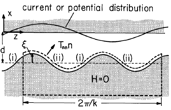
Although not convenient for mathematical derivations, the surface enclosing one periodicity length \(2 \pi/k\) of the rotor, shown in Fig. 4.3.2, helps in understanding how the magnetic traction gives rise to a net force on the rotor. The traction acting normal to the surface has a value \(T_{nn} = \mu_o H_n^2/2\) and hence ispositive. No matter what the excitation from the stator winding, it is clear that at positions (i), where the slope of the stator surface is positive, the magnetic field tends to pull the rotor to the left while at point (ii) the pull is to the right. It is the spatial phase relationship between the stator current distribution and the rotor saliencies that makes one or the other of these forces dominant. It is clear,for example, that if the rotor surface wavelength matched that of the stator current there could be no net force. The z-directed traction acting at any given point would then be cancelled by that acting at a point on the rotor surface a half-wavelength away.
In deriving the relation of the excitation and rotor geometry to the net force, the rotor surface is taken as being at
\[ x = -d + \xi (z,t) = -d + Re \tilde{\xi} \, e^{-j(2k)(z-Ut)} \label{12} \]
The rotor travels with the linear velocity \(U = \omega/k\) and hence its surface, with wavelength \(\pi/k\) half that of the stator excitation, moves in synchronism with the traveling wave of stator surface current:
\[ \overrightarrow{K} = Re \tilde{K}^s e^{j(\omega t - kz)} \overrightarrow{i}_y \label{13} \]
A surface, represented by \(F(x,y,z,t) = x + d -\xi = 0\), has a normal vector
\[ \overrightarrow{n} = \frac{\Delta F}{|\Delta F|} = \frac{\overrightarrow{i}_x - \frac{\partial{\xi}}{\partial{z}} \overrightarrow{i}_z}{|\Delta F|} \label{14} \]
As a reminder that this is a familiar relation, the surface might be one of zero potential \((F \rightarrow \phi)\), with \(\overrightarrow{n}\) the negative of the electric field intensity normalized so that it has unit magnitude. The condition that there be no tangential field on the rotor surface is then
\[ [ \overrightarrow{n} \times \overrightarrow{H}]_y = 0 \rightarrow H_z = -H_x \, \frac{\partial{\xi}}{\partial{z}} \text{at} \, x = -d + \xi \label{15} \]
To match this boundary condition is in general difficult. In this section, it is assumed that \(\xi\) is small,so that Equation \ref{15} is evaluated approximately (to first order in \(\xi\)) at the "equilibrium" position of the rotor surface, \(x = -d\). With \(H_x\) evaluated at \(x = -d\) rather than at \(x = -d + \xi\), the right-hand side of Equation \ref{15} is already written to first order in \(\xi\):
\[ H_z (x = -d + \xi) = H_z (x = -d) + \frac{\partial{H_z}}{\partial{x}} (x = -d) \xi \label{16} \]
If it is further recognized that because \(\overrightarrow{H}\) is irrotational, \(\partial{H_z}/\partial{x} = \partial{H_x}/\partial{z}\), then to first order in \(\xi\), Equation \ref{15} becomes a boundary condition to be evaluated at \(x = -d\), defined as the position \((r)\):
\[ H_z^r = - \frac{\partial{}}{\partial{z}} \, (H_x^r \xi) \label{17} \]
What must be used in evaluating \(H_x^r\) is the zero-order field. This is the field that would be found with \(\xi = 0\), with the rotor presenting a planar surface to a gap excited on the stator side by the current sheet given by Equation \ref{13}. Thus, Equation \ref{17} takes the form
\[ \begin{align} H_z^r &= - \frac{\partial{}}{\partial{z}} \Big [ Re \hat{H}_x^r e^{j(\omega t - kz)} \, Re \hat{\xi} e^{2jk(z-Ut)} \Big ] \nonumber \\ &= - \frac{\partial{}}{\partial{z}} \Bigg \{\frac{1}{2} \Big [\hat{H}_x^r e^{j(\omega t - kz)} + (\hat{H}_x^r)^{*} \, e^{-j(\omega t - kz)} \Big ] \frac{1}{2} \Big [\hat{\xi} \, e^{-2jk(z - Ut)} + \hat{\xi}^{*} \, e^{2jk(z - Ut)} \Big ] \Bigg \} \nonumber \end{align} \label{18} \]
Because of the synchronism condition, \(\omega = kU\), multiplying out this expression gives a term having the same spatial frequency as the stator current and a term at three times that frequency:
\[ H_z^r = - \frac{\partial{}}{\partial{z}} \Bigg [ Re \hat{\psi}_k e^{j(\omega t - kz)} + Re \hat{\psi}_{3k} e^{3j(\omega t - kz)} \Bigg]; \quad \hat{\psi}_k \equiv \frac{1}{2} (\hat{H}_x^r)^{*} \hat{\xi}, \, \hat{\psi}_{3k} \equiv \frac{1}{2} (\hat{H}_x^r) \hat{\xi} \label{19} \]
Note that this expression takes the form \(\overrightarrow{H} = - \Delta \psi\). With the surface \(S_1\) of Fig. 4.2.1a taken as contfguouswith the stator, the desired space-average rotor force is
\[ f_z = A \big \langle T_z \big \rangle_z = A \big \langle \mu_o H_x^s Re \hat{K}^s e^{j(\omega t - kz)} \big \rangle_z \label{20} \]
Note that the terms in Equation \ref{19} are written in the standard complex form, with the quantity in brackets the magnetic potential \(\psi\). The amplitudes at the stator and rotor surfaces (at \(s\) and \(r\)) are therefore related by the transfer relation (Eqs. (a) of Table 2.16.1):
\[ \begin{bmatrix} \mu_o \hat{H}_x^s \\ \mu_o \hat{H}_x^r \end{bmatrix} = \mu_o \, k\begin{bmatrix} -coth \, (kd) & \frac{1}{sinh \, (kd)} \\ -\frac{1}{sinh \, (kd)} & coth \, (kd) \end{bmatrix} \begin{bmatrix} \frac{\hat{K}^s}{jk} \\ \hat{\psi}_k \end{bmatrix} \label{21} \]
for components with dependence \(exp[j(wt -kz)]\) and
\[ \begin{bmatrix} \mu_o H_x^s \\ \mu_o H_s^r \end{bmatrix} = \mu_o \, 3k\begin{bmatrix} -coth \, (3kd) & \frac{1}{sinh \, (3kd)} \\ -\frac{1}{sinh \, (3kd)} & coth \, (3kd) \end{bmatrix} \begin{bmatrix} 0 \\ \hat{\psi}_{3k} \end{bmatrix} \label{22} \]
for components with dependence \(exp 3j(\omega t -kz)\). The infinitely permeable material backing the stator current sheet requires that the third harmonic tangential field at the stator in Equation \ref{22} a vanish.
The normal flux density \(\mu_o H_x^s\) in Equation \ref{20} is a superposition of the components found using Eqs. \ref{21} a and \ref{22} a. Because it multiplies \(\hat{\varepsilon, \hat{H}^r_x\) on the right in these expressions need only be evaluated to zero order in \(\xi\). Thus, \(\hat{H}_x^r\) is given by Equation \ref{21} b with \(\hat{\varepsilon = 0\), and hence \(\hat{\psi}_k = 0\). The second term in Equation \ref{19} also excites a field at the stator surface given by Equation \ref{22} a. But, inserted into Equation \ref{20}, this higher harmonic gives no space-average contribution and hence can be dropped. Thus, Equation \ref{20} becomes
\[ f_z = A \Big \langle Re \, \Bigg \{ j \mu_o \, coth(kd) \, \hat{K}^s + \frac{\mu_o k}{2} \bigg [ \frac{-j (\hat{K}^s)^{*} \hat{\varepsilon}}{ sinh^2 (kd)} \bigg] \Bigg \} e^{j(\omega t - kz)} \, Re \bigg [ \hat{K}^s e^{j(\omega t - kz)} \bigg ] \Big \rangle _z \label{23} \]
The averaging theorem, Eq. 2.15.14, can now be applied to Equation \ref{23} to obtain the first of these relations:
\[ \begin{align} &f_z = \frac{ \mu_o k A}{4 sinh^2 (kd)} Re \big [ (\hat{K}^s)^2 j \hat{\varepsilon}^{*} \big ] \nonumber \quad \quad \quad &f_z = \frac{ -\varepsilon_o k A}{4 sinh^2 (kd)} Re \big [ (k \hat{V}^s)^2 j \hat{\varepsilon}^{*} \big ] \nonumber \end{align} \label{24} \]
The second expression pertains to the electric configuration of Part 4, Table 4.3.1, and has been obtained by recognizing that, in terms of the magnetic and electric potentials, the air-gap fields are analogous.The only difference is that in the magnetic case the stator magnetic potential is \(\hat{K}^s/jk\), while in the electric case, the stator electric potential is \(\hat{V}^s\). Hence, the electric time average force is found (using the complete analogy discussed at the beginning of Sec. 2.16) by replacing \(\mu_o \rightarrow \varepsilon_o\) and is \(\hat{K}^s \rightarrow jk \hat{V}^s\) Equation \ref{24} a to obtain Equation \ref{24} b.
As specific examples having the stator excitations and rotor position when \(t = 0\) shown in Part 4 of Table 4.3.1, let
\[ \varepsilon = \varepsilon_o \, cos \, 2k [ Ut - (z - \delta)] = Re \varepsilon_o \, e^{2jk \delta} \, exp [ 2jk(Ut - z)] \label{25} \]
and
\[ \begin{align} &K^s = K^s_o \, sin (\omega t - kz) = Re (-jK^s_o) \, exp [j (\omega t - kz)] \quad \quad \quad &V^s = V^s_o \, cos (\omega t - kz) = Re V^s_o \, exp [j (\omega t - kz)] \nonumber \end{align} \label{26} \]
where \(\varepsilon_o\), \(K_o^s\) and \(V_o^s\) are taken as real. Then, Eqs. \ref{24} take the specific forms
\[ \begin{align} &f_z = \frac{ -\mu_o k (K_o^s)^2 \varepsilon_o A}{4 sinh^2 (kd)} sin(2k \delta) \quad \quad \quad &f_z = \frac{ -\varepsilon_o k (k V^s_o)^2 \varepsilon_o A}{4 sinh^2 (kd)} sin (2k \delta) \nonumber \end{align} \label{27} \]
The dependence of these forces on the spatial phase of stator excitations and rotor position,sketched in Table 4.3.1, is typical of salient-pole synchronous devices. That \(\langle T_z \rangle_z\) has twice the periodicity in \(k \delta\), obtained with the rotor excited directly by sources having the same periodicity as the stator excitations, is a direct consequence of the induced nature of the magnetization or polarization. Because the surface traction is proportional to the square of the local field the same force is obtained if the rotor is shifted in relative position by \(\delta = \pi/k\). The \([sinh (kd)]^{-2}\) dependence of the force on the gap dimension d results because the only excitation is on the stator. By contrast with the synchronous interactions between excited stators and rotors [with \((d)\) dependence \(sinh(kd)^{-1}\)], here there is a round-trip attenuation of the excitation field, first in reaching the rotor surface and then in being reflected back to the stator.
Of the many configurations in the general family of "salient-pole" devices, two more are shown in Part 5 of Table 4.3.1. The magnetic case is considered in the problems, while the electric one is formally the same as if the rotor were perfectly polarizable. Hence it is also described by Eqs. \ref{24} b and \ref{27} b.
Practical devices make use of large amplitude saliency. One approach to obtaining an appropriate model is developed in Secs. 4.12 and 4.13, where the variable capacitance machine is considered in more detail.