4.6: Kinematics of Traveling-Wave Charged-Particle Devices

Synchronous interactions between a "stator" potential wave and a traveling wave of charge are abstracted in Part 3 of Table 4.3.1. In the most common practical devices exploiting such electric interactions, the space-charge wave is itself created by the electromechanical interaction between a structure potential and a uniformly charged beam. These examples are not "kinematic" in the sense that the relative distribution of space charge cannot be prescribed. Nevertheless, by representing the inter-action as though independent control can be obtained over the beam and structure traveling waves, the energy conversion principles are highlighted. In addition, this section illustrates how the constrained-charge transfer relations of Sec. 4.5 are put to work. Self-consistent interactions through electrical stresses will be developed in Chaps. 5 and 8.

In the model shown in Fig. 4.6.1, the space-charge wave has the shape of a circular cylinder of radius \(R\) and charge density

\[ \rho = - \rho_B \, cos(\omega t - kz + k \delta) = Re \, \tilde{\rho} \, exp(-jkz); \quad \tilde{\rho} \equiv [ -\rho_B \, exp(jk \delta)] \, exp(j \omega t) \label{1} \]

where \(\rho_B\) is a constant.

Fig. 4.6.1. Regions of positive and negative charge represent concentrations and rarefactions in the local charge density of an initially uniformly charged beam moving in the \(z\) direction with the velocity \(U\).

In an electron beam device\(^1\) the stream is initially of uniform charge density. But, perhaps initiated by means of a modulating field introduced upstream, the particles become bunched. The resulting space charge can be viewed as the superposition of uniform and periodic space-charge components. The uniform component gives rise to an essentially radial field which tends to spread the beam. (Through the \(q \overrightarrow{v} \times \overrightarrow{B}\) force attending any radial motion of the particle, a longitudinal magnetic field is often used to confine the beam and prevent its spreading. In any case, here the effect of this radial field is considered negligible.)

In traveling-wave beam devices, the interaction is with a traveling wave of potential on a slow-wave (perhaps helical) structure, such as that shown schematically in Fig. 4.6.2a. The structure is designed to propagate an electromagnetic wave with velocity less than that of light, so that it can be in synchronism with the space-charge wave. For the present purposes, this potential is imposed on a wall at \(r = c\):

\[ \phi_c = V_o \, cos(\omega t - kz) = Re \tilde{V}_o e^{-jkz}; \quad \tilde{V}_o = V_o e^{j \omega t} \label{2} \]

In the kinematic model of Fig. 4.6.1, the coupling can either retard or accelerate the beam, depending on whether operation is akin to a generator or motor (Table 4.3.1). Traveling-wave electron beam amplifiers and oscillators are generators, in that they convert the steady kinetic energy of the beam to an a-c electrical output. The result of the interaction is a time-average retarding force that tends to slow the beam.

Fig. 4.6.2. (a) Schematic representation of traveling-wave electron beam device with slow-wave structure modeled by distributed circuit coupled to beam through the electric field. Below structure is distribution of space charge in the beam (A), and the equivalent distribution of a uniform charge density (B) and a periodic distribution (C). (b) Combination cutaway and phantom view of low-noise low-power traveling-wave tube that operates in part of the frequency range 2 to 40 GHz. (c) Schematic of linear accelerator designed so that oscillating gap voltages "kick" particles as they pass. Shown below are "bunches" of particles and hence space charge (A) and the equivalent superposition of periodic and uniform parts (B) and (C).

The "motor" of particle beam devices is the particle accelerator typified by Fig. 4.6.2c. Here,the object is to accelerate bunches of particles to extremely high velocities by subjecting them to alternating electric fields phased in such a way that when a bunch arrives at an accelerating gap, the fields tend to give it an additional "kick" in the axial direction\(^2\) The complex fields associated with the traveling particle bunches and accelerating fields are typically represented as traveling waves, as suggested by Fig. 4.6.2c. The principal periodic component of the space-charge wave is represented in the model of Fig. 4.6.1.

In this section it is presumed that the particle velocities are unaffected by the interaction; \(U\) is a constant. In fact, the object of the generator is to slow the beam, and of the accelerator is to in-crease the velocity; a more refined analysis is likely to be required for particular design purposes.

In yet another physical situation, the constraints on mechanical motion and wall potentials assumed in this section are imposed. At low frequencies and velocities, it is possible to deposit charge on a moving insulating material. Then, the relative charge velocity is known. Moreover, at low frequencies it is possible to use segmented electrodes and voltage sources to impose the postulated potential distribution.

As will be seen, at low velocities it is difficult to achieve competitive energy conversion densities using macroscopic electric forces. So, at low frequencies, the class of devices discussed in this section might be used as high-voltage generators rather than as generators of bulk power.

The net force on a section of the beam having length \(l\) is found by integrating the stress over a surface adjacent to the outer wall (see Fig. 4.2.1b for detailed discussion of this step):

\[ f_z = 2 \pi a l \langle D_r^c E_z^c \rangle = \pi a l R e [ (\tilde{D}_r^c)^{*} j k \tilde{V}_o] \label{3} \]

To compute \(\tilde{D}^c\), and hence \(f_z\), the potential is related to the normal electric flux and charge density by the transfer relation for a "solid" cylinder of charge, Eq. 4.5.27 with \(m = 0\):

\[ \tilde{\phi}^{\alpha} = \frac{1}{\varepsilon_o} F_o (0, \alpha) \tilde{D}_r^{\alpha} + \sum_{i=0}^{\infty} \frac{\tilde{\rho}_i J_o ( \nu_i \alpha)}{\varepsilon_o (\nu_i^2 + k^2)} \label{4} \]

Table 2.16.2 summarizes \(F_o (0,a)\).

Single-Region Model: It is instructive to consider two alternative ways of representing the fields.First, consider that the beam and the surrounding annular region comprise a single region with a charge density distribution as sketched in Fig. 4.6.3. Then, in Equation \ref{4}, the radius \(\alpha = a\) and the position \((\alpha) + (c)\). Multiplication of Eq. 4.5.19a by \(r \Pi_j (\nu_j r)\) and integration \(0 \rightarrow a\) then gives

\[ \int_o^R \tilde{\rho} r J_o ( \nu_j r) dr = \sum_{i=0}^{\infty} \tilde{\rho}_i \int_o^a r J_o (\nu_i r) J_o (\nu_j r) dr \label{5} \]

Fig. 4.6.3 Radial distribution of charge density.

The right-hand side is integrated using Eq. 4.5.32, while the left-hand side is an integral that can be evaluated from tables or by using the fact that \(J_o(\nu_i r)\) satisfies Eq. 4.5.20 with \(m=0\) and Eq. 2.16.26c holds for \(J_o\):

\[ \tilde{\rho} \frac{R}{\nu_j} J_1 (\nu_j R) = \tilde{\rho}_j \frac{a^2}{2} J_o^2 ( \nu_i a) \rightarrow \tilde{\rho}_i = \frac{2 \tilde{\rho} R J_i ( \nu_i R)}{\nu_i a^2 J_o^2 (\nu_i a)} ; \quad i \neq 0 \label{6} \]

The root \(\nu_i = 0\) to Eq. 4.5.24 is handled separately in integrating Equation \ref{5}. In that case \(J_o = 1\) and \(\tilde{\rho}_o = R^2 \tilde{\rho}/a^2\).

Because \(\tilde{\phi}^c = \tilde{V}_o\), Equation \ref{4} can now be solved for \(\tilde{D}_r^c\);

\[ \tilde{D}_r^c = \varepsilon F_o^{-1} (0,a) \Bigg \{ \tilde{V}_o - \tilde{\rho} \Bigg [ \frac{R^2}{\varepsilon (ak)^2} + \sum_{i=1}^{\infty} \frac{2R J_1 (\nu_i R)}{ \varepsilon \nu_i a^2 (\nu_i^2 + k^2) J_o (\nu_i a)} \Bigg ] \Bigg\} \label{7} \]

It follows from Equation \ref{3} that, for the distribution of charge and structure potential given by Eqs. \ref{1} and \ref{2}, the required force on a length \(l\) of the beam is

\[ f_z = - (\pi R^2l) (k V_o \rho_{\beta} \, sin \, k \delta) L_1 \label{8} \]

where

\[ L_1 = - \frac{a}{R} \Bigg \{ (\frac{R}{a}) \frac{1}{(ak)^2} + \sum_{i=1}^{\infty} \frac{2 J_1 [ (\nu_i a) \frac{R}{a}]}{(\nu_i a)} [ (\nu_ia)^2 + (ak)^2] J_o ( \nu_i a) \Bigg \} a F_o^{-1} (0,a) \nonumber \]

Hence, the force has the characteristic dependence on the spatial phase shift between structure potential and beam space-charge waves identified for synchronous interactions in Sec. 4.3.

Two-Region Model: Consider next the alternative description. The region is divided into a part having radius \(R\) and described by Equation \ref{4} (with the position \(\alpha - e\) and radius \(\alpha + R\)) and an annulus of free space. Because the charge density is uniform over the inner region, only the \(i = 0\) term (having the eigenvalue \(\nu_o = 0\)) in the series of Eq. 4.5.1 is required to exactly describe the charge and potential distributions. With variables labeled in accordance with Fig. 4.6.1, Equation \ref{4} becomes

\[ \tilde{\phi}^e = \frac{D_r^e F_o (0,R)}{\varepsilon} + \frac{\tilde{\rho}{\varepsilon k^2} \label{9} \]

The annular region of free space is described by Eqs. (a) of Table 2.16.2:

\[\begin{bmatrix} \tilde{D}^c_r\\ \tilde{D}^d_r \end{bmatrix} = \varepsilon \begin{bmatrix} f_o (R,a) & g_o (a,R) \\ g_o (R,a) & f_o (a,R) \end{bmatrix} \begin{bmatrix} \tilde{\phi}^c \\ \tilde{\phi}^d \end{bmatrix} \label{10} \]

Boundary conditions splice the regions together:

\[ \tilde{\phi}^c = \tilde{V}_o, \quad \tilde{\phi}^d = \tilde{\phi}^e, \quad \tilde{D}_r^d = \tilde{D}_r^e \label{11} \]

In view of these conditions, Eqs. \ref{9} and \ref{10} b combine to show that

\[ \tilde{\phi}^d = \frac{g_o (R,a) \tilde{V}_o + \tilde{\rho} F_o^{-1} (0,R) \varepsilon^{-1} k^{-2} }{F_o^{-1} (0,R) - f_o (a,R)} \label{12} \]

From Equation \ref{10} a \(\tilde{D}^c_r\) can be found and the force, Equation \ref{3}, evaluated. The result is the same as Equation \ref{8} except that \(L_1\) is replaced by

\[ L_2 = \frac{[ a g_o (a,R) ] [ a F_o^{-1} (0,R)]}{(ka)^2 (\frac{R}{a})^2 [ a F_o^{-1} (0,R) - af_o (a,R)] } = \frac{1}{kR} \, \frac{I_o^{'} (kR)}{I_o (ka)} \label{13} \]

To obtain the second expression, note that the reciprocity condition, Eq. 2.17.10, requires that \(ag_o \, (a,R) = -Rg_o \, (R,a)\).

Numerically, Eqs. \ref{8} and \ref{13} are the same. They are identical in form in the limit where the charge completely fills the region \(r<a\), as can be seen by taking the limit \(R \rightarrow a\) in each expression

\[ L_1 \rightarrow L_2 = - \frac{a F_o^{-1} (0,2)}{(ak)^2} \label{14} \]

In the example considered here the second representation gives the simpler result. But, if the splicing approach exemplified by Equation \ref{13} were used to represent a more complicated radial distribution of charge, the clear advantage would be with the single region representation illustrated by Equation \ref{8}.

Fig. 4.6.4. Function \(L_2\) defined by Eq. 4.6.8.

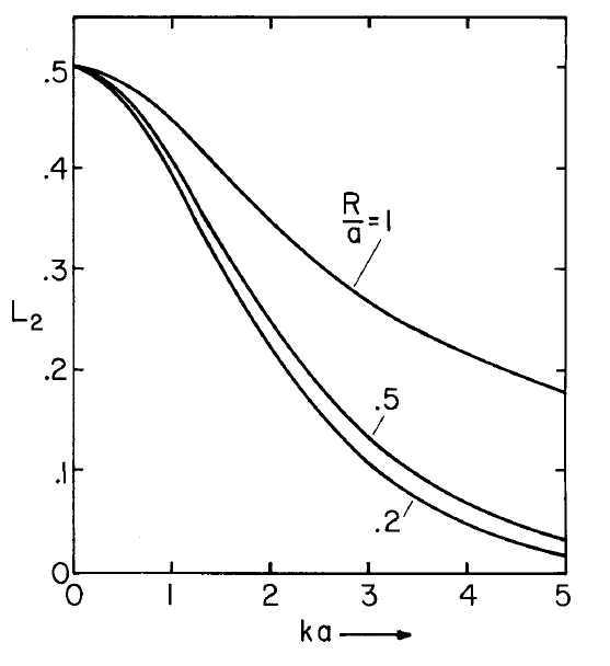
The dependence of \(L_2\) on the wave number normalized to the wall radius is shown in Fig. 4.6.4. As would be expected, the coupling to the wall becomes weaker with increasing \(k\) (decreasing wavelength). The part of the coupling represented by \(L_2\) also becomes smaller as the beam becomes more confined to the center. Note however that there is an \(R^2\) factor in Equation \ref{8} that makes the effect of decreasing \(R\) much stronger than reflected in \(L_2\) (or \(L_1\))alone.

---

1. Basic electron beam electromechanics are discussed in the text Field and Wave Electrodynamics, by Curtis C. Johnson, McGraw-Hill Book Company, New York, 1965, p. 275

2. A discussion of synchronous-type particle accelerators is given in Handbook of Physics, E. U. Condon and H. Odishaw, eds., McGraw-Hill Book Company, New York, 1958, pp. 9-156.