
4.9: Exposed Winding Synchronous Machine Model
- Page ID
- 43854
The structure shown in cross section in Fig. 4.9.1 consists of a stator supporting three windings(a,b,c) and a rotor with a single winding \((r)\). It models a three-phase two-pole synchronous alternator, and is similar to the configuration taken up in Sec. 4.7. The difference is that the windings on both rotor and stator are not embedded in slots of highly permeable material and take up a radial thickness that is appreciable compared to the air gap. As a result, the surface current model used in Sec. 4.7 is not appropriate.
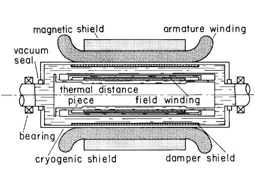
The configuration considered here is an example to which the constrained-current transfer relations of Sec. 4.8 can be applied. It closely resembles models that have been developed for synchronous alternators making use of superconducting field (rotor) windings.\(^1\) With superconductors, it is possible to generate magnetic fields that more than saturate magnetizable materials. As a result, the magnetic materials in which conductors are embedded in conventional machines can be dispensed with. This makes it possible to design for greater voltages than would be possible in a conventional machine, where the slot material in which a conductor is embedded must be grounded. But, because the conductors are exposed to the full magnetic force, methods of construction must be radically altered. A machine built to test approaches to constructing a rotating "refrigerator" required if the field is to be superconducting is shown in Fig. 4.9.2.

In the configuration considered here, it is assumed that surrounding the stator is a highly permeable shield material with inner radius (a) equal to the outer radius of the stator windings. Similarly, the rotor windings are bounded from inside by a "perfectly" permeable core. The magnetic mate-rials are introduced into the model to make the example reasonably free of algebraic complications. In a machine having a superconducting field, a magnetic core would not be used. Development of a model without the magnetic rotor core follows the same pattern as now described.

The distribution of stator and rotor current densities with azimuthal position is shown in Fig. 4.9.3. The turns densities\( (n_a,n_b,n_c ,n_r)\) (conductors per unit area) respectively carry the terminal currents \((i_a, i_b, i_c, i_r)\). The conductors are uniformly distributed. Hence, these current density distributions can be represented by the Fourier series
\[ J_z^s = \Sigma_{m = - \infty}^{+ \infty} \tilde{J}_m^s \, e^{-jm \theta}, \quad b<r<a; \quad J_z^r = \Sigma_{m = -\infty}^{+ \infty} \tilde{J}_m^r \, e^{-jm \theta}, \quad d<r<c \label{1} \]
For the stator winding, the Fourier amplitudes are (Sec. 2.15)
\[ \tilde{J}_m^s = \begin{cases} \frac{2}{\pi m } sin \, (\frac{m \theta_s}{2}) \Bigg [ i_a n_a + i_b n_b e^{\frac{jm \pi}{3}} + i_c n_c e^{\frac{jm 2 \pi}{3}} \Bigg ]; & \text{m odd} \\\\ 0; & \text{m even} \end{cases} \label{2} \]
While on the rotor the amplitudes are
\[ \tilde{J}_m^r = \begin{cases} \frac{2}{\pi m } sin \, (\frac{m \theta_f}{2}) i_r n_r e^{jm \theta_r}; & \text{m odd} \\\\ 0; & \text{m even} \end{cases} \label{3} \]
The constrained-current distribution is now as assumed in the previous section, Eqs. 4.8.4 and 4.8.10.The associated transfer relations relate the Fourier amplitudes of the tangential magnetic field intensities and vector potentials at the surfaces of the annular regions comprising the stator, the air gap and the rotor winding with designations (d) -(j) shown in Fig. 4.9.1.
Boundary Conditions:
There are no surface currents in the model, so the tangential magnetic fields are continuous between regions and vanish on the stator and rotor magnetic materials. The normal flux density is continuous, and this requires that the vector potential be continuous:
\[\begin{align} &\tilde{H}_{\theta m}^d = 0; \, \tilde{H}_{\theta m}^e = \tilde{H}_{\theta m}^f; \, \tilde{H}_{\theta m}^g = \tilde{H}_{\theta m}^h; \tilde{H}_{\theta m}^i = 0 \nonumber \\ & \tilde{A}_m^e = \tilde{A}_m^f; \, \tilde{A}_m^g = \tilde{A}_m^h \nonumber \end{align} \label{4} \]
Bulk Relations:
The transfer relations, Eq. 4.8.12, are now applied in succession to the stator, the air gap and the rotor regions. In writing these expressions, the conditions of Equation \ref{4} are used to eliminate \((e,h)\) variables in favor of the \((f,g)\) variables:
\[ \tilde{A}^d_m = \mu_o G_m(a,b) \tilde{H}_m^f + \mu_o \tilde{J}_m^s h_m(a,b) \nonumber \]
\[\begin{bmatrix} -1 & \mu_o F_m(a,b) & 0 & 0 \\ -1 & \mu_o F_m(c,b) & 0 & \mu_o G_m(b,c) \\ 0 & \mu_o G_m(c,b) & -1 & \mu_o F_m(b,c) \\ 0 & 0 & -1 & \mu_o F_m(d,c) \end{bmatrix} = \begin{bmatrix} \tilde{A}_m^f \\ \tilde{H}_{\theta m}^f \\ \tilde{A}_m^g \\ \tilde{H}_{\theta m}^g \end{bmatrix} = \begin{bmatrix} - \mu_o \tilde{J}_m^s h_m(b,a) \\ 0 \\ 0 \\ -\mu_o \tilde{J}_m^r h_m(c,d) \end{bmatrix} \label{5} \]
\[ \tilde{A}^i_m = \mu_o G_m(d,c) \tilde{H}_{\theta m}^g + \mu_o \tilde{J}_m^r h_m(d,c) \nonumber \]
Because the boundary conditions on the magnetic materials uncouple them from the other relations, the first and last of these relations are written separately.
Torque as a Function of Terminal Variables:
The torque is computed by integrating the Maxwell stress over the surface at \((g)\) on the rotor side of the air gap (sec. 4.2). Because \(B_r = (1/r) (\partial{A}/ \partial{\theta})\),the torque becomes (Eqs. 4.2.3 and 2.15.17):
\[ \tau_z = 2 \pi l c^2 \Sigma_{m = - \infty}^{+ \infty} (\frac{-jm}{c} \tilde{A}_m^g ) (\tilde{H}_{\theta m}^g)^{*} \label{6} \]
To evaluate this expression, the amplitudes \(\tilde{A}_m^g\) and \(H_{\theta m}^g\) are found from the matrix equation of Equation \ref{5}, using Cramer's rule:
\[ \begin{align} &\tilde{A}_m^g = \tilde{J}_m^s C_1 + \tilde{J}_m^r C_2 \nonumber \\ &\tilde{H}_{ \theta m}^g = \tilde{J}_m^s C_3 + \tilde{J}_m^r C_4 \nonumber \end{align} \label{7} \]
Where
\[ \begin{align} &C_1 = \frac{\mu_o^3}{D} h_m (b,a) G_m(c,b) F_m(d,c) \nonumber \\ &C_2 = \frac{\mu_o^3}{D} h_m (c,d) [F_m(a,b) F_m(b,c) – F_m(c,b) F_m(b,c) + G_m(c,b) G_m(b,c)] \nonumber \\ &C_3 = \frac{\mu_o^3}{D} h_m (b,a) G_m(c,b) \nonumber \\ &C_4 = \frac{\mu_o^2}{D} h_m (c,d) [F_m(a,b) - F_m(c,b)] \nonumber \\ &D = \mu_o^2 { G_m(c,b) G_m(b,c) – [F_m(c,b) – F_m(a,b)][F_m(b,c) – F_m(d,c)]} \nonumber \end{align} \nonumber \]
In using Eqs. \ref{7} to evaluate Equation \ref{6}, observe that \(\tilde{J}_m^s (\tilde{J}_m^s)^{*}\) and \(\tilde{J}^r (\tilde{J}_m^r)^{*} \) are even in \(m\), as are also the functions \(h_m, F_m\), and \(G_m\) Because of the latter, the \(C_1\)'s are also even in \(m\). Thus, the summations of the self-field terms in \(|\tilde{J}_m^s|^2\) and \(|\tilde{J}_m^r|^2\) are odd functions of m and result in no contribution. The mth terms are canceled by terms the -mth terms. Only the cross terms appear, as Equation \ref{6} becomes
\[ \tau_z = 2 \pi l c \Sigma_{m = - \infty}^{+ \infty} (-jm) [ \tilde{J}_m^r (\tilde{J}_m^s)^{*} C_2 C_3 + \tilde{J}_m^s (\tilde{J}_m^r)^{*} C_1 C_4] \label{8} \]
Substitution of Eqs. \ref{2} and \ref{3} therefore gives the torque as
\[ \tau_z = \frac{16 l c}{ \pi} i_r n_r \Sigma_{m=1 \\ odd}^{\infty} \frac{C_2 C_3 – C_1 C_4)}{m} sin \, (\frac{m \theta_r}{2}) \, sin \, (\frac{m \theta_s}{2}) [ i_a n_a \, sin \, m \theta_r + i_b n_b \, sin \, m (\theta_r - \frac{\pi}{3}) + i_cn_c \, sin \, m(\theta_r - \frac{2 \pi}{3}) ] \label{9} \]
Where
\[ (C_2 C_3 – C_1 C_4) = \frac{\mu_o^5}{D^2} h_m (c,d) h_m(b,a) G_m(c,b) [ F_m (a,b) F_m(b,c) – F_m(c,b) F_m(b,c) + G_m(c,b) G_m(b,c) + F_m(d,c) F_m(c,b) – F_m(d,c) F_m(a,b) ] \nonumber \]
Electrical Terminal Relations:
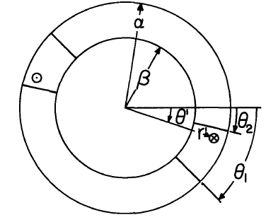
Each of the three phase windings of the stator, as well as the rotor winding, can be represented by the coil shown cross-sectionally in Fig. 4.9.4.For the "a" phase of the stator, variables are identified as \(\theta_1 = \theta_s/2, \, \theta_2 = -\theta_s/2, \, \alpha = a, \, \beta = b\). For the rotor, \(\theta_1 = \theta_r + \theta_f/2, \, \theta_2 = \theta_r - \theta_f/2, \, \alpha = c, \beta = d\).
The flux linked by a single turn of the coil carrying current in the z direction at \((r',\theta^{'})\) and returning it at \((r^{'}, \theta^{'} +\pi)\) is conveniently evaluated in terms of the vector potential (Eq. (f) of Table 2.18.1):
\[ \pi_{\lambda} = l [ A(r^{'}, \theta^{'}) – A(r^{'}, \theta^{'} - \pi)] \label{10} \]
With \(n\) defined as the turns per unit cross-sectional area, there are \(nr^{'}d\theta^{'} dr^{'} \) turns in a differential area and hence the total flux linked by the coil is
\[ \lambda = l \int_{\beta}^{\alpha} \int_{\theta_2}^{\theta_1} \Sigma_{m = - \infty}^{+ \infty} [ \tilde{A}_m (r^{'} e^{-jm \theta^{'}} - \tilde{A}+m (r^{'}) e^{-jm (\theta^{'}- \pi)}] n r^{'} d \theta^{'} dr^{'} \label{11} \]
The integration on \(\theta^{'} \) can be carried out directly to reduce Equation \ref{11} to
\[ \lambda = 2 j l n \Sigma_{m = - \infty \\ odd}^{+ \infty} \frac{ \Big( e^{-jm \theta_1} – e^{-jm \theta_2} \Big)}{m} \int_{\beta}^{\alpha} \tilde{A}_m (r^{'}) r^{'} dr^{'} \label{12} \]
To complete the radial integration, Eq. 4.8.13 is used to express \(\tilde{A}_m\), while for the case being considered \(\tilde{A}_p\) is given by Eq. 4.8.11:
\[ \lambda = 2 j l n \Sigma_{m = - \infty \\ odd}^{+ \infty} \frac{ \Big( e^{-jm \theta_1} – e^{-jm \theta_2} \Big)}{m} [ \tilde{A}_m^{\alpha} M_m (\alpha, \beta) - \tilde{A}_m M_m^{\beta} (\beta, \alpha) - \mu_o \tilde{J} S_m (\alpha, \beta)] \label{13} \]
where
\[ M_m (x,y) = \frac{1}{2} [x^2 - m^2 h_m (x,y)] \nonumber \]
\[ S_m (x,y) = \begin{cases} \frac{x^2}{m^2 - 4} - \frac{y^2}{m^2 - 4} M_m (y,x) - \frac{1}{4} \frac{(x^4 - y^4)}{m^2 - 4}, & \text{m \neq \pm 2} \\\\ - \frac{1}{4} x^2 ln \, x M_m(x,y) + \frac{1}{4} y^2 ln \, y M_m(y,x) + \frac{1}{16} [x^4 (ln \, x - \frac{1}{4}) - y^4 (ln \, y - \frac{1}{4}) ], & \text{m even} \end{cases} \nonumber \]
By appropriate identification of variables, Equation \ref{13} can now be used to compute the flux linked by each of the four electrical terminal pairs. The procedure is illustrated by considering the field winding.Then, variables are identified:
\[ \lambda = \lambda_r, \, d \rightarrow c, \, \beta \rightarrow d, \, \theta_1 = \theta_r - \frac{\theta_f}{2}, \, \theta_2 = \theta_r + \frac{\theta_f}{2}, n = n_r, \tilde{A}^{\alpha} \rightarrow \tilde{A}^g, \, \tilde{A}^{\beta} \rightarrow \tilde{A}^i, \tilde{J} = \tilde{J}_m^r \label{14} \]
The amplitudes \((\tilde{A}_m^g, \tilde{A}_m^i)\) are respectively evaluated from Eqs. 7a and the combination of Eqs. 5f and 7b.Thus, identified with the field winding, Eq. \(13\) becomes
\[ \lambda_r = -\mu_o 4 l n_r \Sigma_{m = -\infty \\ odd} \frac{1}{m} sin (\frac{m \theta_f}{2}) e^{-jm \theta_r} \Big \{ \tilde{J}_m^s [ C_1 M_m (\alpha, \beta) - \mu_o G_m (d,c) C_3 M_m (\beta, \alpha)] + \tilde{J}_m^r [C_2 M_m (\alpha, \beta) - \mu_o G_m (d,c) C_4 M_m (\beta, \alpha) + \mu_o M_m (\beta, \alpha) h_m (d,c) - \mu_o S_m (\alpha, \beta)] \Big \} \label{15} \]
The current density amplitudes are in turn related to the terminal currents by Eqs. \ref{2} and \ref{3}. Thus,Equation \ref{15} is expressed in terms of three mutual inductances and a self-inductance, in the form of Eq. 4.7.3d In writing these inductances, observe that \(F_m\) and \(G_m\) are even functions of \(m\). It follows that \(h_m\) and hence \(M_m\) and \(S_m\) are also even functions of \(m\), and that finally the coefficients of \((\tilde{J}_m^s, \tilde{J}_m^r)\) in Equation \ref{15} are \(m\) summation can be converted to one on positive values of \(m\):
\[\begin{bmatrix} L_{ra} \\ L_{rb} \\ L_{rc} \end{bmatrix} = - \frac{16 l n_r}{\pi} \Sigma_{m=1 \\ odd}^{\infty} \frac{sin (\frac{m \theta_f}{2})}{m} \frac{sin (\frac{m \theta_s}{2})}{m} [ C_1 M_m (\alpha, \beta) - \mu_o G_m (d,c) C_3 M_m (\beta, \alpha)] \begin{bmatrix} n_a \, cos \, m \theta_r \\ n_b \, cos \, m (\theta_r + \frac{\pi}{3}) \\ n_c \, cos \, m(\theta_r + \frac{2 \pi}{3}) \end{bmatrix} \label{16} \]
\[ L_{rr} = - \frac{8 l n^2_r}{\pi} \Sigma_{m = 1 \\ odd}^{\infty} \frac{sin (\frac{m \theta_f}{2})}{m} \frac{sin (\frac{m \theta_s}{2})}{m} [ C_2 M_m ( \alpha, \beta) - \mu_o G_m (d,c) C_4 M_m ( \beta, \alpha) + \mu_o M_m (\beta, \alpha) h_m (d,c) - \mu_o S_m (\alpha, \beta)] \label{17} \]
Because of the energy-conserving nature of the electromechanical coupling, there is redundancy of information in the electrical and mechanical terminal relations. Reciprocity, as expressed by Eq.4.7.32b, can be made the basis for finding the \(\theta_r\) dependent parts of the mutual inductances from the torque, Equation \ref{9}. (Here, there are rotor positions at which each of the mutual inductances vanish, and hence Equation \ref{9} uniquely specifies the mutual inductances.) The reciprocity condition shows that an alternative to the coefficient used to express the mutual inductances in Equation \ref{16} is
\[ [C_1 M_m (\alpha, \beta) - \mu_o G_m (d,c) C_3 M_m (\beta, \alpha) ] = c [ C_2 C_3 - C_1C_4] \label{18} \]
where the quantity on the right is given with Equation \ref{9}.
With the reciprocity relations in view, one efficient approach to determining the complete lumped-parameter terminal relations is to first find the torque, Equation \ref{9}, then use the reciprocity conditions to find the mutual inductances and finally compute the self-inductances from Equation \ref{13}. This last step only requires evaluation of \((\tilde{A}_m^{\alpha},\tilde{A}_m^{\beta})\) with self-current excitations (with currents in other windings removed).
A more conventional approach is to compute the full inductance matrix from Equation \ref{13} and use the lumped-parameter energy method (Sec. 3.5) to find the torque.
1. J. L. Kirtley, Jr., "Design and Construction of an Armature for an Alternator with a Superconducting Field Winding," Ph.D. Thesis, Department of Electrical Engineering, Massachusetts Institute of Technology, Cambridge, Mass., 1971; J. L. Kirtley, Jr., and M. Furugama, "A Design Concept for Large Superconducting Alternators," IEEE Power Engineering Society, Winter Meeting, New York, Jan. 1975.