
4.13: Variable-Capacitance Machines
- Page ID
- 44030
A model for one of the most commonly discussed "electrostatic" synchronous machines (which are themselves rather uncommon) is shown in Fig. 4.12.1a. Both the fixed and moving members have saliency and consist essentially of perfectly conducting material. The time-varying voltage between stator and rotor can either be the source of electrical power for producing a synchronous force in the \(z\) direction on the rotor, or it can serve as the voltage of a bus representing an energy sink for the device acting as a generator. In practice, the stator and rotor members might consist of metallic fins, as shown in Fig. 4.13.1. In the model, regions on the stator and rotor that project into the air gap represent the fins, while regions that dip into the stator and rotor material represent the gaps between fins.


The device is often referred to as a "variable-capacitance" machine because, when the relative position of rotor and stator is such that the projections into the gap are just opposite each other,the capacitance is at a maximum, while it reaches a minimum when the peak in rotor saliency falls just opposite a "valley" in the stator material.
One way to view the energy conversion process is simply to represent the capacitance seen by the voltage source as time-varying. Given the motion of the rotor, the capacitance \(C\) is a known function of time, and the electrical problem comes down to determining a suitable temporal variation for \(C\),relative to a time-varying voltage, \(v\). If power is supplied to the voltage source, it must come from the mechanical forces responsible for making the capacitance vary with time. Thus, the other side of the energy conversion process raises the question: How is a time-average force produced on the rotor by the combination of the salient configuration and the time-varying applied voltage? In this section,we will take up the second question first. What is the electrical force in the direction of motion on the moving member?
The field point of view taken here results in the relation between geometry and capacitance needed to model an actual system, even if the circuit point of view is taken. But also, it makes the example useful in conceptualizing electromechanical interactions that cannot be given a lumped-parameter model. For example, suppose that the undulations on the "rotor" were in fact material de-formations produced by the field itself. This type of self-consistent electromechanical coupling is not kinematic and will be taken up in Chapter 9.
Synchronous Condition
With a sinusoidal voltage \(v(t)\) having period \(T\), applied between the rotor and stator by means of a slip-ring, a time-average electrical force can act in the \(z\) direction on the rotor only if there is a synchronism between the applied voltage and the rotor motion. To this end, consider the physical origins of this force in terms of the model shown in Fig. 4.12.1. Regard-less of the field polarity, at any position on the rotor surface there is an electric force per unit area that is directed perpendicular to the surface and into the air gap. This latter fact makes it clear that without the surface undulations, there can be no electrical force in the \(z\) direction.
To make a synchronous motor, on the time average, fields acting to the right over regions of the rotor surface with a negative slope must produce a greater force than those acting to the left on the regions where the slope is positive. What is the relationship between the excitation period \(T\) and the rotor velocity \(U\) that could result in there being a time-average electrical force? In terms of the displacement \(z_r\) of Fig. 4.12.1, a maximum in the force to the right is obtained with \(z_r\) in the neighborhood of \(\lambda/4\). Thus, with the rotor in this position, the applied \(v^2\) should be at its maximum. By the time the rotor is at \(z_r = 3 \lambda / 4\), the force produced is in the wrong direction, and hence \(v^2\) should be near a null. By the time \(z_r = 5 \lambda /4, \, v^2\) should be peaking again. It is concluded that in the time \(T/2\), the rotor should move one wavelength: \(UT/2 = \lambda\). Thus, the synchronism condition is met if
\[ z_r = Ut + \delta; \, U = \frac{ 2 \lambda}{T} \label{1} \]
Here, \(\delta\) is a spatial phase-angle determined by the mechanical load on a motor or the electrical load on a generator.
The quasi-one-dimensional electric field is given by Eqs. 4.12.7 and 4.12.9 un-normalized:
\[ E-x = \frac{v}{d + \xi_s - \xi_r}; \, E-z = (x + d) \frac{\partial{E_x}}{\partial{z}} - \frac{\partial{}}{\partial{z}} (\xi_r E_x) \label{2} \]
The force on a section of the rotor one wavelength long and \(a\) length \(l\) in the \(y\) direction is found by integrating the Maxwell stress tensor over an enclosing surface as pictured in Fig. 4.2.1a. The only surface giving a contribution is the one of constant \(x\) in the air gap:
\[ f_z = l \int_{z}^{z+ \lambda} \varepsilon_o E_x E_z dz \label{3} \]
This integral can be evaluated using the fields of Equation \ref{2}. That it does not matter what \(x = constant\) plane is used in carrying out the integration (except for physical reasons, to have the assurance that the surface does not cut through one of the electrode inward peaks) is evident from the fact that
\[ \int_z^{z + \lambda} \varepsilon_o E_x (x+d) \frac{\partial{E_x}}{\partial{z}} dz = \varepsilon_o (x+d) \int_{z}^{z + \lambda} \frac{\partial{}}{\partial{z}} (\frac{1}{2} E_x^2) dz = \varepsilon_o (x+d) [ E_x^2 (z + \lambda) - E_x^2(z) ] = 0 \label{4} \]
The final deduction follows from the spatial periodicity of the structure. The remaining contributions to the integral are expressed using the normalization
\[ z = \lambda \underline{z}, \, \xi_s = d \underline{\xi}_s, \, \xi_r = d \underline{\xi}_r, \, \delta = \lambda \underline{\delta}, \, z_r = \lambda \underline{z}_r \label{5} \]
With \(f_z \equiv ( \varepsilon_o l v^2/d) \underline{f}_z\), Equation \ref{3} becomes
\[ f_z = - \int_{z}^{z+1} \frac{1}{1 + \xi_s - \xi_r} \frac{\partial}{\partial{z}} \Big [ \frac{\xi_r}{1+ \xi_s - \xi_r} \Big ] dz \label{6} \]
Carrying out the differentiation in the integrand gives
\[ f(z_r) \equiv - \int_{z}^{z+1} \frac{ (1 + \xi_s) \frac{\partial{\xi_r}}{\partial{z}} - \xi_r \frac{\partial{\xi_s}}{\partial{z}}}{ (1 + \xi_s - \xi_r)^3} dz \label{7} \]
Once the integral is completed, the function \(f\) depends on the amplitudes of \(\xi_s\) and \(\xi_r\) and on the irrelative displacement \(z_r\). The time-average force is then computed by specifying this relative displacement in terms of Equation \ref{1}. In normalized variables, with \(t = T \underline{t}\)
\[ \bigg \langle f_z \bigg \rangle_t = \frac{\varepsilon_o l }{d} \int_{\underline{t}}^{\underline{t} + 1} v^2 (\underline{t}) \underline{f} (2 \underline{t} + \underline{delta}) d \underline{t} \label{8} \]
As an example, consider stator and rotor electrodes having sinusoidal shapes of equal amplitude and a sinusoidal excitation voltage (note that Eqs. \ref{7} and \ref{8} are general in regard to these specifications):
\[ \underline{\xi}_s = \underline{\xi}_o cos \, 2 \pi \underline{z}, \, \underline{\xi}_r = \underline{\xi}_o cos \, 2 \pi (\underline{z} -\underline{z}_r), \, v(t) = V cos \, 2 \pi \underline{t} \label{9} \]
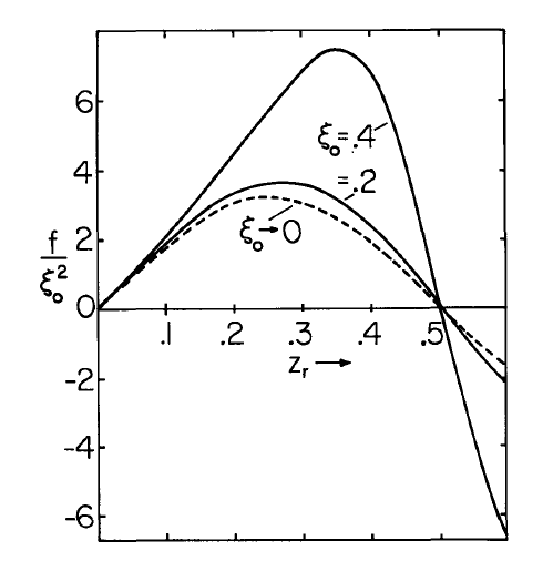
Numerical integration of Equation \ref{7} then gives the dependence on relative displacement and amplitude shown in Fig. 4.13.2a. To highlight the nonlinear effects of \(\xi_o, \, f\) is normalized to \(\xi_o^2\) so that much of the dependence on the electrode amplitudes is suppressed.
The electrodes make their closest approach to each other with \(\underline{z}_r = 0.5\) and are furthest a part when \(\underline{z}_r = 0\). Thus, for a given voltage, the fields tend to be more intense in the range \(0.25<\underline{z}_r<0.5\) than they are in the range \(0<\underline{z}_r<0.25\).This nonlinear effect is reflected in the tendency of the force to be skewed toward relative deflections in the former range. As would be expected from the singularity in the denominator of Equation \ref{7}, as the electrodes tend to touch \((\underline{\xi}_o \rightarrow 0.5)\), the force tends to approach infinity just to the left of \(\underline{z}_r = 0.5\). The function \(f(z_r)\) is then used to numerically integrate Equation \ref{8}, with the result the normalized time-average force shown as a function of relative displacement phase \(\delta\) and amplitude \(\underline{\xi}_o\) in Fig. 4.13.2b. Again, the dependence on \(\underline{\xi}_o\) is partially suppressed in the normalization.
The electromechanical model exemplified by Eqs. \ref{7} and \ref{8} is nonlinear, in the sense that the electrode deflections can be of arbitrary amplitude in the range \(0.25<\underline{\xi}_o<0.5\). The fact that the time-average force becomes infinite as \(\underline{\xi}_o \rightarrow 0.5\) is to be expected. At some instant, the electrodes are then at the point of touching and the associated field is becoming extremely large where the electrodes are nearly in contact. (Physically, electrical breakdown would of course present a limit on the validity of the theory.) Within the validity of an air-gap dielectric that does not permit electrical breakdown, the procedure which has been followed is an example of the left vertical leg in Fig. 4.12.2.
Further linearization, based on \(\xi_s << d\) and \(\xi_5 << d\), demonstrates what is meant by a "linearized quasi-one-dimensional" model and by the completion of the step represented by the lower horizontal leg in Fig. 4.12.2.
For small amplitudes, \((1 + \xi_s - \xi_r)^{-3} \simeq 1 - 3 ( \xi_s - \xi_r)\), and hence Equation \ref{7} becomes
\[ f(z_r) \rightarrow \int_{z}^{z+1} [ (1+ \xi_s) \frac{\partial{\xi_r}}{\partial{z}} - \xi_r \frac{\partial{\xi_s}}{\partial{z}} - 3(\xi_s - \xi_r) \frac{\partial{\xi_r}}{\partial{z}} + ...] dz = \xi_o \pi sin \, 2 \pi z_r \label{10} \]

(In carrying out this and the next integration it is helpful to represent the expressions of Equation \ref{9} in complex notation and make use of the averaging theorem, Eq. 2.15.14.) In turn, the time average called for by Equation \ref{8} can now be evaluated:
\[ \bigg \langle f_z \bigg \rangle_t = \frac{ \varepsilon_o l V^2 \underline{\xi}_o^2 \pi}{d} \int_{\underline{t}}^{\underline{t} + 1} cos^2 \, 2 \pi \underline{t} \, sin \, 2 \pi (2 \underline{t} + \underline{\delta}) d \underline{t} \label{11} \]
Carrying out this integration gives
\[ \bigg \langle f_z \bigg \rangle_t = ( l \lambda) \bigg [ \varepsilon_o (\frac{V}{d})^2 \bigg ] \frac{d}{\lambda} (\frac{\xi_o}{d})^2 \frac{\pi}{4} sin (\frac{2 \pi \delta}{\lambda}) \label{12} \]
This approximation to the time-average force is shown by the broken curve of Fig. 4.13.2b.
Note that the small-amplitude force of Equation \ref{12} takes the form of the area \(l \lambda\) multiplied by the electric pressure \(\varepsilon_o (V/d)^2\) times factors representing the fraction of this product obtained by dint of the geometry and the relative phase of the rotor and the driving voltage.
The variable-capacitance machine is closely related to the salient-pole machine described in Sec. 4.3 (Case 4b of Table 4.3.1). In that example, the stator is "smooth" with electrodes con-strained by a traveling wave of potential. The effect of having a stator with saliencies driven by a simple voltage source (which is likely to be more convenient) is to produce a similar time-average force.
Linearized from the outset, the variable-capacitance machine of this section could also be viewed in terms of an interaction between the rotor traveling wave and one of two stator waves, the sum of which is equivalent to the physical stator structure considered. The result of such an analysis would be a model without restrictions as to the gap width relative to the wavelength. For the related example of Sec. 4.3,. Eq. 4.3.27b retains information (represented by the denominator, \(sinh^2(kd))\)about the effect of the air gap in the limit where \(d\) becomes large. This result, restricted to small amplitude but valid for arbitrary air-gap spacing, is typical of the amplitude parameter expansion or linearization modeling step of Fig. 4.12.2. Taking the long-wave limit for the example from Sec. 4.3 constitutes taking the limit of Eq. 4.3.27b, \(kd<< 1\). Following this route of first linearizing and then taking the long-wave limit for the variable-capacitance machine considered in this section is an alternative derivation of Equation \ref{12}, and is considered in the problems.