
5.5: Impact Charging of Macroscopic Particles - The Whipple and Chalmers Model
- Page ID
- 28149

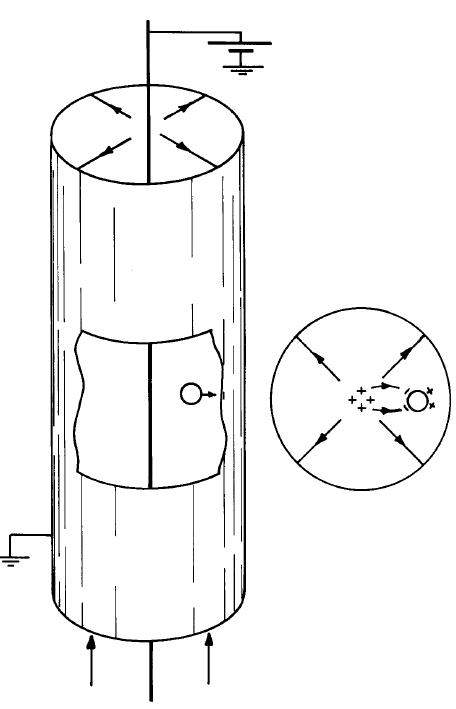
Electrostatic precipitators, used for the collection of particulate from gases in air-pollution control systems, make use of ion impact charging. A typical configuration is shown in Fig. 5.5.1. Dust laden gas enters the metallic tube from the bottom, and the object is to separate the dust from the gas before the latter leaves at the top. The high-voltage wire supported at the center of the tube sustains a corona discharge, a type of electrical breakdown that remains localized around the wire. Within this corona discharge, both positive and negative ions are created. Positive ions are drawn outside the immediate vicinity of the corona where they migrate along the lines of force toward the grounded co-axial electrode.
A particle of dust that interrupts the electric field also interrupts the ion migration. As a result the particle becomes charged.
Once charged,it too is subject to an electrical force and hence also tends to migrate to the cylindrical wall. The final stage of particle collection consists in rapping the electrode so that compacted dust falls from the walls into a hopper below.\(^1\)
Provided that the contribution of the migrating ions to the electric field in the immediate vicinity of the particle is negligible, the model developed in this section describes the charging process. As the particle acquires charge, its own contribution to the field is altered, so this example gives the opportunity to exemplify the quasistationary migration presaged in Sec. 5.3.
Typical electric fields in an electrostatic precipitator are \(5 x 10^5 \, V/m\). Thus, ions having a mobility of about \(2 x 10^{-4} \, (m/sec)/(V/m)\) have velocities \(bE \simeq 100 \, m/sec\). Typical gas velocities are only \(1-2 \, m/sec\), so the effects of convection on the charging process are usually not significant.
But convection is an important factor in other situations to which the impact charging model pertains. It is well known that as drops of water fall through the atmosphere, they become charged because of interactions with ions. In a thunderstorm, a system of ions and drops can be subject to a significant electric field.
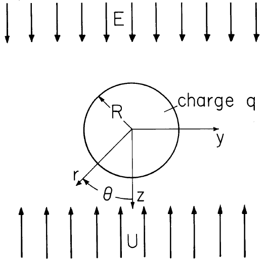
The particle shown in Fig. 5.5.2 is taken as spherical with an "imposed" electric field E that is locally uniform and if positive directed as shown. As envisioned by meteorologists, the particle is a water drop falling through the atmosphere, so from the frame of reference of the particle, there is an ambient gas velocity U directed upward in the \(-z\) direction.For the meteorologist the question is, given ions of a certain density carried by the combined field and flow,what is the charging law for the particle? How fast does it become charged and to what final value? Whipple and Chalmers \(^2\) were interested in a quantitative model of Wilson's theory of thunderstorm electrification,which centered around how a particle could acquire charge while falling through essentially equal densities of positive and negative ions.\(^2\)
In the following discussion, the particle being charged will be called the "drop," while the impacting particles will be termed ions. In fact, the"ions" might be fine macroscopic particulate being collected (scrubbed) by charged drops\(^3\).At the outset, two useful parameters are identified. Regimes of charging are demarked by the critical charge
\[ q_c \equiv 12 \pi \varepsilon_o R^2 E \label{1} \]
which can be positive or negative, depending on the sign of \(E\). Rates of charging will be characterized by the currents
\[ I_{\pm} = \pi R^2 b_{\pm} \rho_{\pm} E = q_c \frac{b_{\pm} \rho_{\pm}}{\varepsilon_o 12} \label{2} \]
That the charging rate is to be calculated implies that the electric field and hence the ion motions are not in the steady state. However, as discussed in Sec. 5.3, it is assumed that ion transit times through several particle radii \(R\) are short compared to charging times of interest. Hence, at any instant the particle charge is taken as a known constant, which then makes a contribution to the instantaneous electric field intensity.
The particle is taken as perfectly conducting. The electric potential is therefore constant at \(r = R\), becomes \(-E_o r cos \theta\) far from the particle and is consistent with there being a net charge \(q\) on the particle. The appropriate combination of the potentials (satisfying Laplace's equation, as discussed in Sec. 2.16) \(r \, cos \, \theta, cos \, \theta/r^2\) and \(q/4 \pi \varepsilon_o r\) therefore is the "imposed" field:
\[ \overrightarrow{E} = - \nabla \phi = { E (\frac{2R^3}{r^3} +1) \, cos \, \theta + \frac{q}{4 \pi \varepsilon_o r^2}} \overrightarrow{i}_r + { E (\frac{R^3}{r^3} - 1) sin \, \theta } \overrightarrow{i}_{\theta} \label{3} \]
It follows from this result and Eq. 5.3.8a that the "stream" function for the electric field intensity is
\[ \Lambda_E = ER^2 [ \frac{R}{r} + \frac{1}{2} (\frac{r}{R})^2] \, sin^2 \, \theta - \frac{q \, cos \, \theta}{4 \pi \varepsilon_o} \label{4} \]
The velocity distribution in the neighborhood of the particle must have both tangential and normal components that vanish on the particle surface, and must approach the uniform flow at infinity. Written in terms of a stream function, in accordance with Eq. 5.3.8b, the velocity distribution automatically is solenoidal (the flow is incompressible). Conservation of momentum supplies the additional law to determine the velocity distribution, but there is no exact analytical solution valid for all velocities. As is shown in Sec. 7.20, if forces due to viscosity dominate those due to inertia, Stokes's flow around a sphere applies, and the associated stream function is (from Eqs. 7.20.13 and 7.20.17)
\[ \Lambda_v = \frac{-UR^2}{2} [ (\frac{r}{R})^2 - \frac{3}{2} (\frac{r}{R}) + \frac{1}{2} \frac{R}{r}] sin^2 \, \theta \label{5} \]
The flow field found by using Eq. 5.3.8b is valid, provided the Reynolds number (Sec.7.20) \(R_y = \rho R U / \mu < 1\), where \(\mu\) is the fluid viscosity. A fifty micron radius water droplet in free fall through air has \(R_y \simeq 0.7\).
Given Eqs. \ref{4} and \ref{5}, the characteristic lines are determined by substituting into Eq. 5.3.13b to obtain
\[ \frac{1}{2} \frac{U}{b_{\pm} E} [ (\frac{r}{R})^2 + \frac{1}{2} (\frac{R}{r}) - \frac{3}{2} (\frac{r}{R})] sin^2 \, \theta \pm [ \frac{R}{r} + \frac{1}{2} (\frac{r}{R})^2] sin^2 \, \theta \pm \frac{3q}{q_c} \, cos \, \theta = C \label{6} \]
The upper and lower signs, respectively, refer to positive and negative migrating particles and \(C\) is a constant which identifies the particular characteristic line.
Just what constant charge density should be associated with each of these lines is determined by a single boundary condition imposed wherever the line "enters" the volume of interest.In terms of parameters now introduced, the object is to obtain the net instantaneous electrical current to the particle, \(i_{+}(q,E,U,\rho_{+})\). With the imposed field, velocity and charge densities held fixed, this expression then serves to evaluate the drop rate of charging
\[ \frac{dq}{dt} = i_{\pm} (q) \label{7} \]
Permutations and combinations of flow velocity, imposed field, instantaneous drop charge, and sign of the incident particles are large, so an orderly approach is required to sort out the possible collection regimes. These are conveniently pictured in the \((q,bE)\) plane: for positive particles Fig. 5.5.3,for negative ones Fig. 5.5.4.
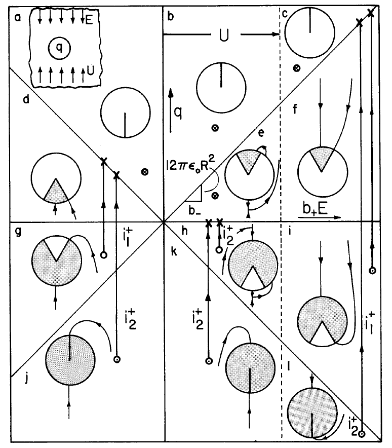
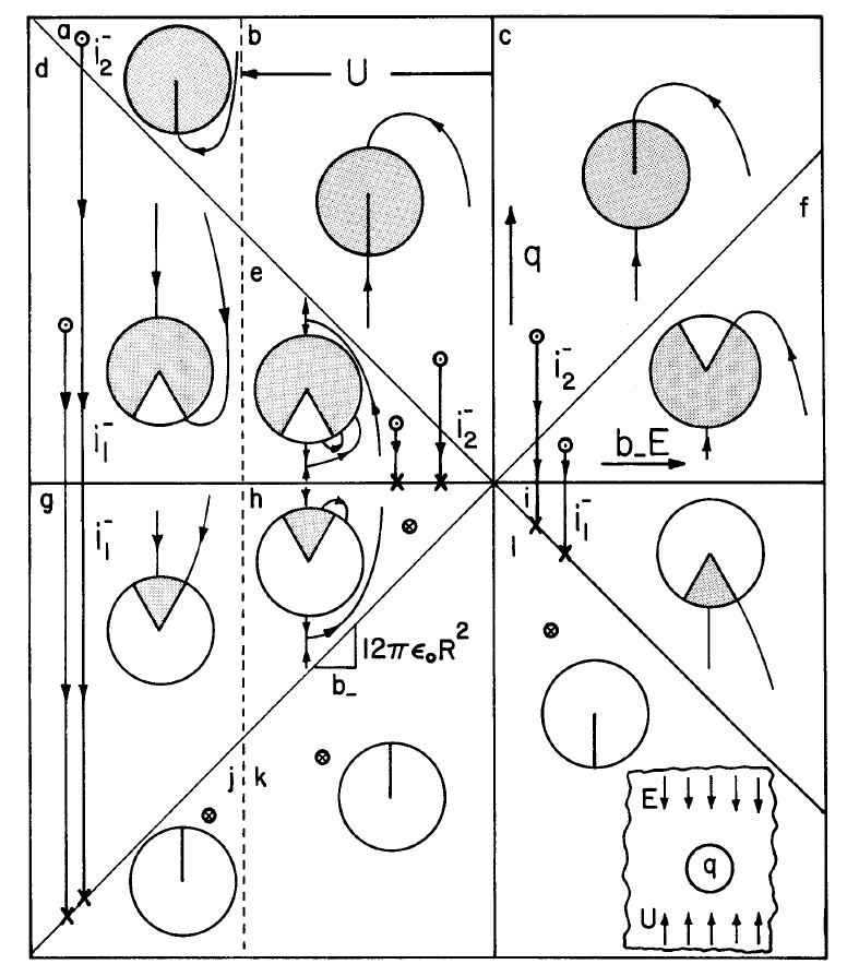
First, recognize the surfaces which satisfy the condition of Eq. 5.3.6, and hence at which boundary conditions on the charge density are imposed. For positive particles (upper sign) and b+E > U the distribution of particle densities for particles entering at \(z \rightarrow - \infty\) is required. Otherwise, the charge density is imposed as \(z \rightarrow + \infty\) because the positive particles enter from below. These conditions therefore respectively apply to the left and right of the line \(b_{+}E = U\) in Fig. 5.5.3. Characteristic lines originating on the particle surface carry zero charge density. Also, at the particle surface the normal fluid velocity is zero; hence the characteristic lines degenerate to \(\pm b_{\pm} \overrightarrow{E}\). This greatly simplifies the charging process, because the electric field intensity given by Eq.\ref{3} can be used to decide whether or not a given point on the particle surface can accept charge. Evaluation shows that characteristic lines are directed into the particle surface wherever
\[ \theta_c < \theta < \pi \quad \begin{cases} \text{positive ions}, & E > 0 \\ \text{negative ions}, & E < 0 \end{cases} \label{8} \]
\[ 0 < \theta < \theta_c; \quad \begin{cases} \text{positive ions}, & E < 0 \\ \text{negative ions}, & E > 0 \end{cases} \label{9} \]
where the critical angle, \(\theta_c\), demarking regions of inward and outward force lines, follows from the radial component of Equation \ref{3} evaluated at \(r = R\):
\[ cos \, \theta_c = - \frac{q}{q_c} \label{10} \]
A graphical representation of what has been determined is given by the direction of incident force lines on the particle surfaces sketched in Figs. 5.5.3 and 5.5.4. Where directed inward, these force lines indicate a possible electric current density. Whether or not the current is finite depends on whether the given characteristic line originates elsewhere on the drop boundary or at infinity.
In any case, if a characteristic line is directed outward, there is no charging current density to the particle, and so without further derivations, regimes \((a)\), \((b)\) and \((c)\) for the positive particles (Fig. 5.5.3) and \((j)\), \((k)\) and \((Z)\) for the negative particles (Fig. 5.5.4) give no charging current. From Equation \ref{7}, within these regimes the drop charge remains at its initial value.
Regimes (f) and (i) for Positive Ions; (d) and (g) for Negative Ions
To continue the characterization of each regime shown in Figs. 5.5.3 and 5.5.4, upper and lower signs respectively will be used to refer to the positive and negative ion cases.
The characteristic line terminating at the critical angle on the drop surface reaches the \(z \rightarrow -\infty\) surface at the radius \(y^{*}\) shown in the respective regimes in the Fig. 5.5.3. Particles entering within that radius strike the surface of the drop within the range of angles wherein the drop can accept ions.Hence, to compute the instantaneous drop charging current, simply find this radius \(y^{*}\) and compute the total current passing within that radius at \(z \rightarrow -\infty\). The particular line is defined by Equation \ref{6} evaluated at the critical angle, and on the particle surface: \(\theta = \theta_c\), \(r = R\). Thus, the constant is evaluated as
\[ C = \pm \frac{3}{2} [1 + (\frac{q}{q_c})^2] \label{11} \]
To find \(y^{*}\), take the limit of Equation \ref{6} \((r \rightarrow \infty, \, y^{*} = (r \, sin \, \theta) \text{and} \, cos \, \theta \rightarrow -1 ))\ using the constant of Equation \ref{11} to determine that
\[ (y^{*})^2 (1 \pm \frac{U}{b \pm E}) = 3R^2 [1- \frac{q}{q_c}]^2 \label{12} \]
The current passing through the surface with radius \(y^{*}\) is simply the product of the current density and the circumscribed area:
\[ i_1^{\pm} = \pm n_{\pm} q_{\pm} (\pm b_{\pm} E - U) \pi (y^{*})^2 \label{13} \]
The combination of Eqs. \ref{12} and \ref{13} is
\[ i_1^{\pm} = 3 I_{\pm} (1 - \frac{q}{q_c})^2 = \pm 3 |I_{\pm}| \, (1 \pm \frac{q}{|q_c|})^2 \label{14} \]
The second equality is written by recognizing the sign of E in the respective regimes.
In the positive ion regimes \((f)\) and \((i)\), the charging current is positive, tending to increase the drop charge until it reaches the limiting value \(q = |q_c|\). Charging trajectories are shown in the figures, with \(i_1\) the rate of charging, whether the initial drop charge is within the respective regimes or the charge passes from another regime into one of these regimes, and then passes on to its final value, \(|q_c|\).For example, in the case of the positive ion charging, it will be shown that a drop charges at one rate in regime \((l)\) and then, on reaching regime \((i)\), assumes the charging rate given by Equation \ref{14}, which it obeys until the charge reaches a final value on the boundary between regimes \((f)\) and \((c)\).
Also sketched in Figs. 5.5.3 and 5.5.4 are the characteristic lines, and the critical angles defining those portions of the drop over which conduction can occur. As a drop charges and then passes from regime \((i)\) to \((f)\), and finally to the boundary between regimes \((f)\) and \((c)\) in the positive particle case, the angle over which the drop can accept particles decreases from a maximum of \(2 \pi\) to \(\pi\) at \(q = 0\),and finally to zero when \(q = |q_c|\). It is the closing of this "window" through which charge can be accepted to the particle surface which limits the drop charge to the critical or "saturation" value \(q_c\).
Regimes (d) and (g) for Positive Ions; (f) and (i) for Negative Ions
These regimes are analogous to the four just discussed except that the particles enter at \(z \rightarrow \infty\), rather than at \(z \rightarrow -\infty\). The derivation is therefore as just described except that the limiting form of Equation \ref{6} is taken as \(\theta + 0\), with \(C\) gain given by Equation \ref{11} to obtain
\[ (y^{*})^2 (1 \pm \frac{U}{b_{\pm} E}) = 3 R^2 (1 + \frac{q}{q_c})^2 \label{15} \]
Then, the particle currents can be evaluated as
\[ i_1^{\pm} = -3 I_{\pm} (1 + \frac{q}{q_c})^2 = \pm 3 |I_{\pm}| (1 \pm \frac{q}{|q_c|})^2 \label{16} \]
As would be expected on physical grounds, the positive ion case gives charging currents and final drop charges in regimes \((d)\) and \((g)\) which are the same as those in \((f)\) and \((i)\).
Regimes (j) and (k) for Positive Ions; (b) and (c) for Negative Ions
For these regimes, the total surface of the drop can accept particles. The radius for the circular cross section of ions reaching the surface of the drop from \(z \rightarrow \infty\) is determined by the line intersecting the drop surface at \(\theta = \pi\). This line is defined by evaluating Equation \ref{6} at \(r = R, \theta = \pi\) to obtain
\[ C = \pm \frac{3q}{q_c} \label{17} \]
Then, if the limit is taken \(r \rightarrow \infty, \, \theta \rightarrow 0\), of Equation \ref{6}, \(y^{*}\) is obtained and the current can be evaluated as
\[ i_2^{\pm} = \pm n_{\pm} q_{\pm} (\mp b_{\pm} E + U) \pi (y^{*})^2 = \frac{12 |I_{\pm}|}{|q_c|} a \label{18} \]
Note that in the positive ion regimes,\(q\) is negative, so the result indicates that the particle charges at this rate until it leaves the respective regimes when the charge \(q = -|q_c|\).
Regime (k) for Positive Ions; (a) for Negative Ions
The situation here is similar to that for the previous cases, except that ions enter at \(z \rightarrow - \infty\), so the appropriate constant for the critical characteristic lines given by Equation \ref{6} evaluated at \(r = R, \, \theta = 0\), is the negative of Equation \ref{17}. The limit of that equation given as \(r \rightarrow \infty , \, \theta \rightarrow \pi\), gives \(y^{*}\) and evaluation of the current gives a value identical to that found with Equation \ref{18}. In regime \((k)\), for positive particles, where the initial charge is negative, the charging current is positive, and tends to reduce the magnitude of the drop charge until it enters regime \((i)\), where its rate of charging shifts to iI and it continues to acquire positive charge until it reaches the final value \(|q_c|\) indicated on the diagram.
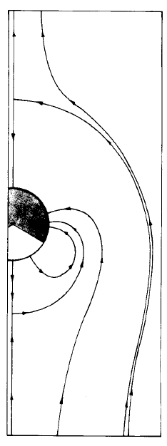
Regime (e), Positive Ions; Regime (h), Negative Ions
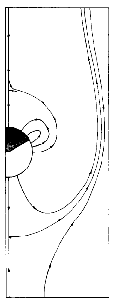
In regimes \((e)\) and \((h)\) for either sign of particles, the window through which the drop can accept a particle flux is on the opposite side from the incident particles. Typical force lines are drawn in Fig. 5.5.5. Force lines terminating within the window through which the drop can accept ions can originate on the drop itself. In that case, the charge density on the characteristic line is zero, since the drop surface is incapable of providing particles.
To determine the particle charge that just prevents force lines originating at \(z \rightarrow \infty\) from terminating on the particle surface, follow a line from the \(z\) axis where the drops enter at infinity back to the drop surface. That line has a constant determined by evaluating Equation \ref{6} with \(\theta = 0\)
\[ C = \pm \frac{3q}{q_c} \label{19} \]
Now, if Equation \ref{6} is evaluated using this constant, and \(r = R\), an expression is found for the angular position at which that characteristic line meets the drop surface
\[ \frac{3}{2} \, sin \, \theta = \frac{3q}{q_c} \, (cos \, \theta - 1) \label{20} \]
Note that the quantity on the right is always negative if \(q/q_c\) is positive, as it is in regimes \((e)\) for the positive particles and \((h)\) for the negative. Thus, in regime \((e)\) for the positive particles and \((h)\) for the negative, the rate of charging vanishes and the drop remains at its initial charge.
Regime (h) for Positive Ions; (e) for Negative Ions
In these regimes, \(q/q_c\) is negative and Equation \ref{20} gives an angle at which the characteristic line along the \(z\) axis meets the drop surface. Typical force lines are shown in Fig. 5.5.6. To compute the rate of charging, the solution to this equation is not required because a circular area of incidence for ions at \(z \rightarrow \infty\) is then determined by the characteristic line reaching the drop at \(\theta = \pi\). Actually, no new calculation is necessary because that radius is the same as that found for regime \((k)\) for the positive ions and \((b)\) for the negative. The charging current is \(i_2^{\pm}\), as given by Equation \ref{18}. Drops in these regimes discharge until they reach zero charge. Moreover, if the initial drop charges place the drop in regimes \((k)\) for the positive ions or \((b)\) for the negative ions, the rate of discharge follows the same law through regimes \((h)\) for the positive ions and \((e)\) for the negative until the drop reaches zero charge.
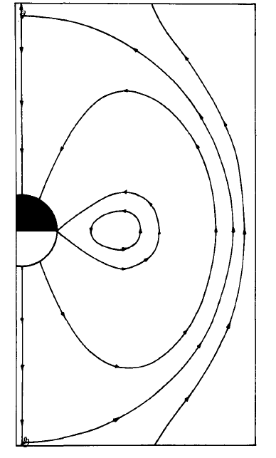
As a matter of interest, in regimes \((e)\) and \((h)\) for both positive and negative ions a doughnut-shaped island of closed force lines is attached to the critical line if \(0.5 < |bE|/U < 1\). An illustration is Fig. 5.5.7.
Positive and Negative Particles Simultaneously
If both positive and negative particles are present simultaneously, the drop charging is characterized by simply superimposing the results summarized with Figs. 5.5.3 and 5.5.4. (The independence of species migration is discussed in Sec. 5.3.) The diagrams are superimposed with their origins(marked 0) coincident. A given point in either plane then specifies the drop charge and associated field experienced by both families of charges. This justifies superimposing the respective currents at the given point to find the total charging current:
\[ \frac{dq}{dt} = i_{+}(q) + i_{-}(q) \label{21} \]
Here,\(i_{+}\) is \(i_1^{+}, i_2^{+}\) or \(0\), in accordance with the charging regime and similarly, \(i_-\) is the appropriate current due to negative ions.
Drop Charging Transient
The quasistationary charging process is illustrated specifically by considering the fate of a drop starting out in regime \((l)\) of Fig. 5.5.3, in a field \(b_{+}E > U\) and with a for charge \(q < -|q_c|\). Then, Equation \ref{7} with \(i_2^{+}\) given by Equation \ref{18}, becomes
\[ \int_{q_o}^q \frac{dq}{q} = - \int_o^t \frac{12 |I_+|}{|q_c|} dt = - \int_o^t \frac{\rho_+ b_+}{\varepsilon_o} dt \label{22} \]
where \(q_o\) is the drop charge when \(t = 0\). Thus, so long as the charge remains in regime \((l)\), the charging transient is
\[ q = q_o e^{-t/\tau}; \, \tau \equiv \varepsilon_o/ \rho_+ b_+ \label{23} \]
When the drop has been discharged to \(q = -|q_c|\), the rate of discharge switches to \(i_1^+\), given by Equation \ref{16}. Thus, the charging equation is
\[ \int_{-q_c}^q \frac{dq}{(I \mp \frac{q}{|q_c|})^2} = \pm 3 |I_{\pm}| \int_o^{t'} dt' \label{24} \]
where \(t'\) is the time measured relative to when the drop switches into regime \((i)\). Integration gives a charging transient
\[ q = |q_c| \Bigg (\frac{t'/4 \tau - \frac{1}{2}}{t'/4 \tau + \frac{1}{2}} \Bigg ) \label{25} \]
which completes the discharging of the drop and goes on in regime \((f)\) to charge the drop positively until it approaches the saturation charge \(q_o\).
Note that although the detailed temporal dependence of Eqs. \ref{23} and \ref{25} is quite different, the same charge relaxation time \(\varepsilon_o/\rho_+b_+\) characterizes the charging dynamics. It is this time that must be long compared to the particle transient time to justify the quasistationary model. The same time constant has a second complementary significance, brought out in the next section. There, it is possible to appreciate the relation of space-charge effects to the quasistationary model used in this section.
1. H. J. White, Industrial Electrostatic Precipitation, Addison-Wesley Publishing Company, Reading,Mass., 1963, pp. 33-48.
2. F. J. W. Whipple and J. A. Chalmers, "On Wilson's Theory of the Collection of Charge by Falling Drops," Quart. J. Roy. Meteorol. Soc. 70, 10
3. (1944).3. J. R. Melcher, K. S. Sachar and E. P. Warren, "Overview of Electrostatic Devices for Control of Submicrometer Particles," Proc. IEEE 65, 1659 (1977).