5.7: Collinear Unipolar Conduction and Convection- Steady D-C Interactions

The electrohydrodynamic coupling undertaken in this section illustrates the electromechanical energy conversion processes that can take place if the space charge density is large enough to provide a significant contribution to the electric field. In the configuration shown in Fig. 5.7.1, a pair of electrically conducting grids at \(z = 0\) and \(z = l\) provide electrical "terminals" through which the fluid can pass and by which entrained charge particles are either injected or collected. The grids have the potential difference \(v\). Charged particles are injected with zero potential at \(z = 0\) and collected at potential \(v\) on the grid at \(z = l\). Hence, with a load attached to the terminals, the charge carried by the fluid results in a current through the load, so that the configuration converts mechanical energy to electrical form. In this case, the fluid plays the role of the belt in a Van de Graaff generator.In fact, as for the Van de Graaff machine described in Sec. 4.14, it will be seen that generator, pump (motor) and brake operation are all possible.

Fig. 5.7.1One-dimensional unipolar d-c pump, generator or brake.

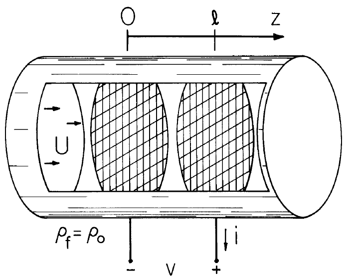
There is an important difference between the collinear configuration considered here and the Van de Graaff machine. In the latter, the generated field is orthogonal to the field associated with the charge carried by the belt. Here, transverse dimensions are very large and the charge entrained in the fluid produces a field that i4 collinear with the "generated" or "imposed" field associated with charges on the grids. Thus, \(\overrightarrow{E} = \overrightarrow{i}_z E(z) \). As a result, the electromechanical energy conversion is through normal stresses, rather than shear stresses. The volume between the grids can be identified with the volume shown in the abstract by Fig. 4.15.1, or specifically by Fig. 5.7.2.

Fig. 5.7.2 The fluid volume between the grids is subject to the mechanical normal stresses (pressure) \(p\) defined as positive if acting inward.

Interest is confined to steady-state conditions, so conservation of charge, represented by Eq. 5.2.2 with \(G-R = 0\) and \((\partial{p}/\partial{t}) = 0\), requires that the current density be solenoidal. The fluid is incompressible, sa that \(\overrightarrow{v}\) is also solenoidal. It follows from the one-dimensional model that the fluid velocity \( \overrightarrow{v} = U \overrightarrow{i}_z\) and the current density \(\overrightarrow{J} = \overrightarrow{i}_z J\), where \(U\) and \(J\) are independent of \(z\):

\[ J = \frac{i}{A} = \rho (bE + U) \label{1} \]

The scale of interest is presumed large enough that effects of diffusion are negligible.

In addition to Equation \ref{1}, Gauss' law relates \(\rho\) to \(\overrightarrow{E} = \overrightarrow{i}_z E(z)\). Elimination of \(E\) between these equations gives

\[ \rho^{-1} d \rho^{-1} = \frac{b}{\varepsilon J} dz \label{2} \]

If the charge is injected with density \(\rho(0) = \rho_o\), Equation \ref{2} is integrated to give

\[ \frac{\rho}{\rho_o} = \Big (1 + \frac{2}{R_e} \frac{i_o}{i} \frac{z}{l} \Big )^{-1/2} \label{3} \]

where \(i_o \equiv \rho_o U A\) and the electric Reynolds number \(R_e \equiv U \varepsilon/b \rho_o l\). Note that \(R_e\) is the ratio of the charge relaxation time \(\varepsilon/b \rho_o\) (based on the charge density at the entrance) to the fluid transport time \(l/U\). Hence, if \(R_e\) is large, convection plays a dominant role in determining the charge distribution.

Now, if Equation \ref{3} is used with Equation \ref{1}, the electric field intensity is known:

\[ E \equiv \frac{U}{b} \Big \{ \frac{i}{i_o} \bigg [1 + \frac{2}{R_e} \frac{i_o}{i} \frac{z}{l} \bigg ]^{1/2} - 1 \Big \} \label{4} \]

and integration of \(E\) in turn gives the potential distribution

\[ \phi = \frac{Ul}{b} \Big \{ \frac{z}{l} - \frac{R_e}{3} (\frac{i}{i_o})^2 \bigg [ \big (1 + \frac{2}{R_e} \frac{i_o}{i} \frac{z}{l} \big )^{3/2} - 1 \bigg ] \Big \} \label{5} \]

Thus, because \(\phi(l)\) is the terminal voltage \(v\), the "volt-ampere" characteristic of the device has been obtained.

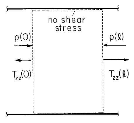
The pressure rise \( \Delta p \equiv p(l) -p(0)\) is balanced by the net electrical force on the fluid. Hence it is simply the difference in the normal electric stresses evaluated at the outlet and inlet. From Equation \ref{4}

\[ \Delta p = \frac{\varepsilon}{2} [ E^2 (l) - E^2(0) ] = \frac{\varepsilon U^2}{2 b^2} \Bigg \{ \Big [ \frac{i}{i_o} \Big (1 + \frac{2i}{R_e i} \Big )^{1/2} -1 \Big ] ^2 - \Big [ \frac{i}{i_o} - 1 \Big ] ^2 \Bigg \} \label{6} \]

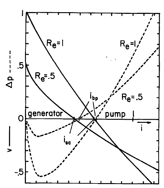
The pump, brake and generator energy conversion regimes can be identified by considering the dependence of the electrical power out, \(P_e = vi\), and of the mechanical power in, \(P_m = -\nabla p UA\), on the normalized current \(i/i_o\). These dependences are shown in Fig. 5.7.3 with the electric Reynolds number, \(R_e\), as a parameter. Note that as Re is raised, the \(v-i\) relationship approaches that of a current source with \(i = i_o\) (a vertical line through \(i/i_o = 1\) on the plot). The short-circuit current i_{sc}, normalized to \(i_o\), is determined by \(R_e\). From Equation \ref{5} evaluated at \(z = l\) and with \(v = 0\),

\[ R_e = \frac{3 (4r^2 - 3) + [9 (4r^2-3)^2 - 192r^3 (r-1)]^{1/2}}{12 r^2 (1-r)}; \, r \equiv \frac{i_{sc}}{i_o} \label{7} \]

For convenience, \(R_e\) is expressed here as a function of \(i_{sc}/i_o\). The current \(i_{bp}\) (at which the pressure rise is zero) follows from Equation \ref{6}:

\[ i_{bp}/i_o = 2 R_e/ (2R_e +1) \label{8} \]

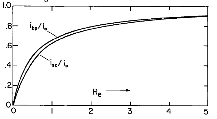
These currents \(i_{sc}\) and \(i_{bp}\) are sketched as a function of \(R_e\) in Fig. 5.7.4. They demark the extremes of the brake regime of operation, and hence also define the upper and lower currents, respectively, of the generator and pump regimes.

Fig. 5.7.3. Electrical and mechanical terminal characteristics as a function of the normalized terminal current with the electric Reynolds number \(R_e\) as a parameter. \(v\) is normalized to \(\rho_o l^2/ \varepsilon\), \(\Delta p\) is normalized to \((\rho_p l)^2/2 \varepsilon\), and \(i\) to \(i_o\).

Fig. 5.7.4. Dependence of the normalized short-circuit and zero-pressure-drop currents on the electric Reynolds number \(R_e\).

 

The Generator Interaction

The optimum generator performance, from the point of view of electrical breakdown, is obtained by making \(E(l) = 0\), so that the maximum pressure change is obtained for a given maximum \(E\). In this case, it follows from Eq. \ref{4} that \(i/i_o\) should be adjusted to make

\[ \frac{i}{i_o} = - \frac{1}{R_e} + [(1/R_e)^2 + 1]^{1/2} \label{9} \]

In any case, the electrical power output is given by Eq. \ref{5} as

\[ P_e = vi = \frac{\rho_o A U^2 l}{b} (\frac{o}{i_o}) \big \{1 - \frac{R_e}{3} (\frac{i}{i_o})^2 [(1 + \frac{2}{R_e} \frac{i_o}{i})^{3/2} - 1] \big \} \label{10} \]

For this particular case, the mechanical power input follows from Eqs. \ref{6} and \ref{9} as

\[ P_m = - \Delta p UA = \frac{U^3 A \varepsilon}{2b^2} (\frac{i}{i_o} -1)^2 \label{11} \]

From these last two expressions, an electromechanical energy conversion efficiency is determined as a function of \(R_e\) or \(i/i_o\):

\[ \frac{P_e}{P_m} = \frac{1}{3} (1+ 2 \frac{i}{i_o}) = \frac{1}{3} \big \{ 1 - \frac{2}{R_e} + 2[(1/R_e)^2 +1]^{1/2} \big \} \label{12} \]

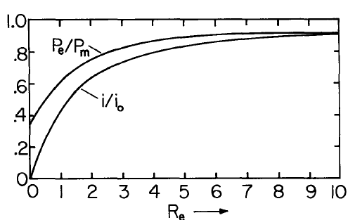
The dependences of the energy conversion efficiency and \(i/i_o\) on \(R_e\) are summarized in Fig. 5.7.5.

 

The Pump Interaction

Consider now the distribution of fields that gives rise to the greatest pressure rise for a given maximum electric field intensity within the flow. From Eq. 6, in this case \(E(0) =0 \): a condition obtained by making \(i = i_o\).That is, at the entrance current is entirely carried by the convection, there being no slip velocity between the charge carriers and the neutral fluid.The electrical power \(P_e\) is again given by Eq. \ref{10}, but now \(i/i_o = 1\). The mechanical power \(P_m\) follows from Eq. \ref{6} and the current condition as

\[ P_m = - \frac{U^3 A \varepsilon}{2b^2} [(1+ 2/R_e)^{1/2} - 1]^2 \label{13} \]

The efficiency of the electrical to mechanical energy conversion is then fully determined by the electric Reynolds number

\[ \frac{P_m}{P_e} = 3 [ 2 (1+2/R_e)^{1/2} + 1]^{-1} \label{14} \]

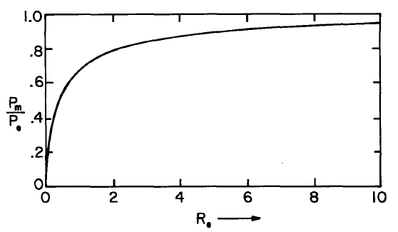
The dependence on \(R_e\) is summarized in Fig. 5.7.6.

Fig. 5.7.5 Dependence of generator electromechanical energy conversion efficiency \(P_e/P_m\) and normalized terminal current \(i/i_o\) on the electric Reynolds number \(R_e\).

Fig. 5.7.6 Efficiency of electrical to mechanical energy conversion for unipolar one-dimensional interaction with current \(i=i_o\) that the entrance electric field intensity is zero.

Fig. 5.7.7. Distribution of charge density and electric field intensity for generator and pump. The parameter \(R_e \equiv (\varepsilon/b \rho_o)/(l/U) \) can be regarded as a normalized velocity.

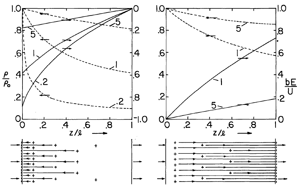
For both the generator and pump under these idealized conditions, the charge and electric field distributions are illustrated in Fig. 5.7.7. Because the relationship between \(i/i_o\) and \(R_e\) is determined by the operating conditions (Eq. \ref{9} for the generator and \(i/i_o = 1\) for the pump) the only parameter is \(R_e\).

In this steady-state interaction, characteristics, emphasized in Sec. 5.6, still offer an alternative point of view. In the neighborhood of a given charged particle as it passes through the inter-action region, the charge density must decay in accordance with Eq. 5.6.2. The spatial rate of decay shown in Fig. 5.7.7 decreases with increasing electric Reynolds number because the particle then spends less time in the interaction region.