5.14: An Electroquasistatic Induction Motor; Von Quincke's Rotor

The configuration of Fig. 5.14.1 gives the opportunity to study charge relaxation for finite-thickness conductors. Regions (a) and (b) are each composed of homogeneous materials having uniform conductivity and permittivity. The \(b-c\) interface moves to the right with a uniform velocity, \(U\). The materials may move as rigid bodies with this same velocity, or might be composed of fluids which have some unspecified velocity profile \(\overrightarrow{v} = v_z(x) \overrightarrow{i}_z\). They are bounded from below by a constant-potential plane, and from above by a system of electrodes used to impose a traveling wave of potential.

An objective is to determine the fields and hence the electrical surface force density acting on the interface in the direction of motion. From Sec. 5.10 it is known in advance that the only charges within the moving materials exist where the conductivity and permittivity have a spatial variation, at the interface. The planar configuration could be a developed model for a system "closed on itself" so that the interaction considered would be between a system of rotating, semi-insulating materials and an imposed rotating electric field. Except for geometric factors, the torque on the semi-insulating rotor sketched in Fig. 5.14.2 depends on the physical parameters and the imposed fields in essentially the same way as for the planar case study (see Problem 5.14.1).

The potential is the given traveling wave at the boundary denoted by (a), is continuous at the interface, and must vanish at the lower boundary \((\hat{\phi}^a = \hat{V}_o, \, \hat{\phi}^b = \hat{\phi}^c, \, \hat{\phi}^d = 0)\). Thus, the transfer relations representing the field distributions in the bulk of each region, Eqs. (a) of Table 2.16.1, are

\[\begin{bmatrix} \hat{D}_x^a \\ \hat{D}_x^b \end{bmatrix} = \begin{bmatrix} - \varepsilon_a k coth(ka) & \frac{\varepsilon_a k}{sinh(ka)} \\ \frac{-\varepsilon_a k}{sinh(ka)} & \varepsilon_a k coth(ka) \end{bmatrix} \begin{bmatrix} \hat{V}_o \\ \hat{\phi}^b \end{bmatrix} \label{1} \]

\[\begin{bmatrix} \hat{D}_x^c \\ \hat{D}_x^d \end{bmatrix} = \begin{bmatrix} - \varepsilon_b k coth(kd) & \frac{\varepsilon_b k}{sinh(kb)} \\ \frac{-\varepsilon_b k}{sinh(kb)} & \varepsilon_b k coth(kb) \end{bmatrix} \begin{bmatrix} \hat{\phi}^b \\ 0 \end{bmatrix} \label{2} \]

By contrast with the model used in Sec. 5.13, there is no surface conduction, but rather a volume conduction, so that the boundary condition implied by conservation of charge for the interface,

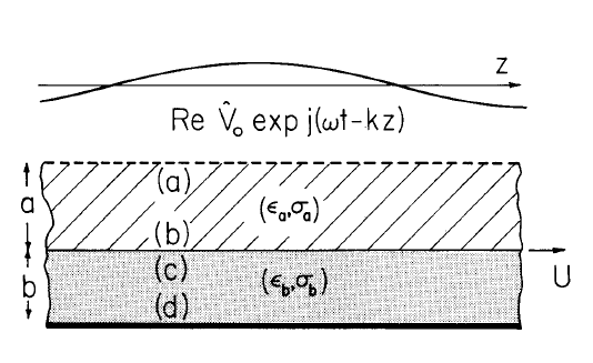
Fig. 5.14.1. Cross-sectional view of two planar layers of material having thicknesses \(a\) and \(b\), respectively. The potential is constrained to be a traveling wave just above, and to be constant just below.

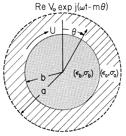
Fig. 5.14.2. Circular analog of the planar system of Fig. 5.14.1. Qualitatively, fields in the planar problem are the same as those in this circular configuration if the \(z\) axis of Fig. 5.14.1 is wrapped around on itself in an integral number of wavelengths.

and represented by Eq. 5.12.4, becomes

\[ \Big ( \frac{\sigma_a}{\varepsilon_a} \hat{D}_x^b - \frac{\sigma_b}{\varepsilon_b} \hat{D}_x^c \Big ) + j (\omega - kU) (\hat{D}_x^b - \hat{D}_x^c) = 0 \label{3} \]

The space average of the surface force density acting on the only charges within the volume of interest, those at the interface, is given by integrating the Maxwell stresses over an incremental volume enclosing the interface and having one wavelength in the \(z\) direction (see Sec. 4.2 for a similar calculation).Thus, the space-average force per unit area is

\[ \langle T_z \rangle _z = \frac{1}{2} Re [ (\hat{D}_x^b)^{*} \hat{E}_z^b - (\hat{D}_x^c)^{*} \hat{E}_z^c] = \frac{1}{2} Rejk \hat{\phi}^b (\hat{D}_x^b - \hat{D}_x^c)^{*} \label{4} \]

The jump in \(D_x\) called for with Eq. \ref{4} is the surface charge density given by subtracting Eq. \ref{2}a from \ref{1}b:

\[ \hat{D}_x^b - \hat{D}_x^c = \frac{-\varepsilon_a k \hat{V}_o}{sinh(ka)} + \hat{\phi}^b k [ \varepsilon_a coth(ka) + \varepsilon_b coth(kb)] \label{5} \]

Then, substitution into Eq. \ref{4} shows that it is the interfacial potential which determines the space-average of the surface force density

\[ \langle T_z \rangle_z = - \frac{\varepsilon_a k^2}{2 \, sinh(ka)} \, Rej \hat{\phi}^b \hat{V}_o^{*} \label{6} \]

With the objective of finding \(\hat{\phi}^b\), the first quantity in brackets in Eq. \ref{3} is found in terms of the potential \(\hat{\phi}^b\) by multiplying Eq. \ref{1}b by \(\sigma_a/ \varepsilon_a\) and subtracting Eq. \ref{2}a multiplied by \(\sigma_b/\varepsilon_b\):

\[ \frac{\sigma_a \hat{D}_x^b}{\varepsilon_a} - \frac{\sigma_b \hat{D}_x^c}{\varepsilon_b} = \frac{-\sigma_a k}{sinh(ka)} \hat{V}_o + \hat{\phi}^b k [ \sigma_a coth(ka) + \sigma_b coth(kb)] \label{7} \]

Then, substitution of Eqs. \ref{5} and \ref{7} into \ref{3} gives the required surface potential in terms of the driving potential

\[ \hat{\phi}^b = \frac{[j (\omega - kU) \varepsilon_a + \sigma_a] \hat{V}_o}{sinh(ka) \{ [ \sigma_a coth(ka) + \sigma_b coth(kb)] + j (\omega - kU) [ \varepsilon_a coth(ka) + \varepsilon_b coth(kb)] \}} \label{8} \]

For purposes of physical interpretation, it is helpful also to have the surface charge density given in terms of the driving potential by substituting Eq. \ref{8} into Eq. \ref{5}:

\[ \hat{D}_x^b - \hat{D}_x^c = \frac{-k \hat{V}_o coth(kb) (\varepsilon_a \sigma_b - \varepsilon_b \sigma_a)}{sinh (ka) [ \sigma_a coth(ka) + \sigma_b coth(kb)] (1+ jS_E)} \label{9} \]

where

\[ S_E = \omega \tau_E ( 1 - \frac{kU}{\omega}), \, \tau_E = \frac{[ \varepsilon_a coth(ka) + \varepsilon_b coth(kb)]}{[\sigma_a coth(ka) + \sigma_b coth(kb)]} \label{10} \]

Finally, the electric surface force density is found by substituting Eq. \ref{8} into Eq. \ref{6}:

\[ \langle T_z \rangle _z = \frac{1}{2} \varepsilon_a (k \hat{V}_o) (k \hat{V}_o)^{*} K (\varepsilon_a \sigma_b - \varepsilon_b \sigma_a) \frac{S_E}{1 + S_E^2} \label{11} \]

where 

\[ K = coth(kb)/ \{ sinh^2 (ka) [ \varepsilon_a coth(ka) + \varepsilon_b coth(kb)] [ \sigma_a coth(ka) + \sigma_b coth(kb)] \} \nonumber \]

What has been computed relates to a number of different physical situations. If the material layers are solid, then Eq. \ref{11} represents the force per unit \(x-y\) area acting on the layers. Even though Eq. \ref{11} came from an integration of the stresses over a volume enclosing only the interface, because there is no free charge density anywhere else in the volume of the materials, it includes all of the force on the material. It is possible that one or the other, or both, of the materials could be fluids,in which case Eq. \ref{11} is the surface force density acting at the interface and \(U\) is the interfacial velocity. The calculation remains correct, even if the material to either side of the interface moves with some velocity other than \(U\).

To examine the physical implications of Eq. \ref{11}, suppose that the traveling-wave frequency is fixed, and interest is in the dependence of the electrical surface force density on the material velocity. First, note that for a given \(kU/ \omega\), the sign of the surface stress depends on the relative permittivities and conductivities. If the lower material is sufficiently more conducting than the upper one, so that \(\sigma_b \varepsilon_a > \sigma_a \varepsilon_b\), then for \(kU/\omega < 1\) the force is in the same direction as the wave velocity. As a function of \(S_E\), this stress first rises linearly, reaches a peak, and then falls off, in a manner familiar from Sec. 5.13. The dependence on \(U\) has the same nature except that the point where \(S_E\) vanishes is at the synchronous velocity \(U = \omega/k\), and increasing \(U\) is equivalent to decreasing \(S_E\). Hence, a plot of \(\langle T_z \rangle _z\) as a function of the normalized velocity \(kU/\omega\) is as shown in Fig. 5.14.3. If the lower material is a conducting solid or fluid, and the intervening material an insulator, such as air, and the interface moves at a velocity less than synchronous, there is an induced electrical force tending to pull the material in the direction of wave propagation.

If the electrical force is retarded by one proportional to the velocity, as would be the case with viscous damping, then the velocity at which there would be an equilibrium between the electrical force and the retarding viscous force is the intersection (i) of Fig. 5.14.3a. The material tends to follow the traveling wave at a somewhat lesser velocity than the phase velocity \(\omega/k\). Note that, if a perturbing force makes the velocity decrease in magnitude slightly, the electrical force dominates the viscous force and tends to return the material to its steady equilibrium position. An experiment illustrating the force as it pumps a liquid is shown in Fig. 5.14.4a.

So far, there is little qualitative difference between what has been found for the finite-thick-ness slab and the results of Sec. 5.13 for the sheet conductor. But now, suppose that the material adjacent to the traveling-wave structure conducts sufficiently more than that below so that \(\sigma_a \varepsilon_b > \sigma_b \varepsilon_a\),From Eq. \ref{11}, it is clear that the electrical force now acts in a direction which opposes the direction of relative propagation for the field. Even more, there are now three velocities at which the electrical force can be equilibrated by a viscous retarding force. At position (ii), the material is moving in a direction opposite to that of the wave.

Arguments similar to those given for equilibrium (i) can be used to see that (ii) is also stable.Two equilibria are possible with the material moving faster than the traveling wave. Of these, (iii)is unstable and (iv) is stable.

The example illustrates that there are exceptions to the intuitive notion that in an induction type of interaction, the material always tends to follow the traveling wave, and that under conditions of "motor" operation, the material velocity is less than the phase velocity of the wave.

The seemingly mysterious finding, with \(\sigma_a \varepsilon_b > \varepsilon_a \sigma_b\), is explained first by considering why the material follows the traveling wave in the case of Fig. 5.14.3a. Equation \ref{9} gives the surface charge density, and shows that there is negative surface charge lagging the peak in potential on the electrode above by an angle less than \(90^o\). The picture is one of a field axis on the fixed structure pulling along charges induced in the material. But, if the material adjacent to the electrodes is the conductor, so that \(\sigma_a \varepsilon_b > \varepsilon_a \sigma_b\), then Eq. \ref{9} shows that the sign of the charge at the interface is reversed. Regions of positive charge on the electrodes induce positive surface charge on the adjacent interface. What was a force of attraction in the case of Fig. 5.14.3a, becomes a force of repulsion in Fig. 5.14.3b. This is why the material can actually be repelled in a direction opposite to that of the traveling wave. An illustrative experiment is shown in Fig. 5.14.4b.

Equilibrium (iii) is best illustrated by considering the limit where the applied frequency vanishes. Thus, the applied potential is static. In the circular analog of Fig. 5.14.2 the applied field might be produced by a pair of parallel plates used to impose a field perpendicular to the z axis that, in the absence of the conducting materials, would be uniform. Such a configuration is Von Quincke's rotor,illustrated in Fig. 5.14.4c. The rotor is insulating relative to the corn oil in which it is immersed; hence \(\varepsilon_a \sigma_b < \varepsilon_b \sigma_a\). The electrical force then depends on the material velocity, as sketched in Fig. 5.14.3c. If the applied field is raised, then there is a threshold value of field at which the slope of the electric force curve exceeds that of the viscous force. At that condition, equilibrium(iii) becomes unstable and the material spontaneously moves, in the developed model either to the right or left, in the circular geometry clockwise or counterclockwise, so as to establish a new equilibrium with a steady-state velocity either at (ii) or (iv). At the position (iii), the static field induces positive charges on the interface directly opposite positive charges on the electrodes. As a result,any small excursion of the material which tends to carry that charge distribution to the right or left is accompanied by a proportionate electric stress that tends to further the original deflection.

Spontaneous rotation of insulating objects immersed in somewhat conducting media and stressed by \(d-c\) fields are observed in seemingly unrelated situations. Examples are macroscopic particles in semi-insulating liquids and objects in ionized gases.