5.15: Temporal Modes of Charge Relaxation

Temporal Transients Initiated from State of Spatial Periodicity

The configurations of the two previous sections are typical of linear systems that are inhomogeneous in one direction only and excited from transverse boundaries. Pictured in the abstract by Fig. 5.15.1, the transverse direction, \(x\), denotes the direction of inhomogeneity, while in the longitudinal (\(y\) and \(z\)) directions the system is uniform. In Secs. 5.13 and 5.14, it is at transverse boundaries (having \(x\) as the perpendicular) that driving conditions are imposed. In the transverse picture, \(\phi_d\) imposes a driving frequency \(\omega\) and a spatial dependence on the longitudinal coordinates that is periodic, either a pure traveling wave with known wavenumbers \((k_y,k_z)\) or a Fourier superposition of these waves. The most common configuration in which spatial periodicity is demanded is one in which \(y\) or \(z\) "closes on itself," for example becomes the \(\theta\) coordinate in a cylindrical system.

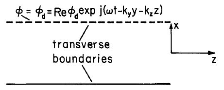
Fig. 5.15.1. Abstract view of systems that are inhomogeneous in a transverse direction, \(x\), and uniform in longitudinal directions \((y,z)\).

The temporal transient resulting from turning on the excitation when \(t = 0\) with the system initially at rest can be rep-resented as the sum of a particular solution (the sinusoidal steady-state driven response) and a homogeneous solution (itself generally the superposition of temporal modes having the natural frequencies \(s_n\)):

\[ \phi(x,y,z,t) = Re \hat{\phi} (x) e^{j(\omega t - k_y y - k_z z)} + \Sigma_n Re \hat{\phi}_n (x) e^{s_n t - j(k_y y + k_z z)} \label{1} \]

Turning off the excitation results in a response composed of only the temporal modes. The coefficients conditions for all \(\phi_n(x)\) are adjusted to guarantee that the total response satisfy the proper initial values of \(x\). In some situations this may require only one mode, whereas in others an infinite set of modes is entailed.

Identification of the eigenfunctions and their associated eigenfrequencies is accomplished in one of two ways. First, if the driven response is known, its complex amplitude takes the form

\[ \hat{\phi}(x) = \frac{\hat{\phi}_d}{D(\omega, k_y, k_z)} \label{2} \]

By definition, the natural modes are those that can exist with finite amplitude even in the limit of zero drive. This follows from the fact that the particular solution in Eq. \ref{1} satisfies the driving conditions, so the natural modes must vanish at the driven boundaries. Thus, for given wavenumbers \((k_y,k_z)\) of the drive, the frequencies \(s_n\) must satisfy the dispersion relation

\[ D(-j s_n, k_y, k_z) = 0 \label{3} \]

Alternatively, if it is only the natural modes that are of interest, then the amplitudes are required to satisfy all boundary conditions, including those implied by setting the excitations to zero. In the abstract system of Fig. 5.15.1, \(\phi_d = 0\).

The natural modes identified in this way are only those that can be excited by means of the structure on the transverse excitation boundary. Thus, the implied distributions of sources within the volume are not arbitrary. The functions \(\hat{\phi}_n (x)\) are complete only in the sense that they can be used to represent arbitrary initial conditions on sources induced in this way. They are not sufficient to rep-resent any initial distribution of the fields set up by some other means within the volume. The remainder of this section exemplifies this subject in specific terms. Magnetic diffusion transients, considered in Chapter 6, broaden the class of example.

 

Transient Charge Relaxation on a Thin Sheet

The build-up or decay of charge on a moving conducting sheet excited by a sinusoidal drive can be described by revisiting the example treated in Sec. 5.13. In terms of the complex amplitude of the sheet potential, \(\hat{\phi}^b\), and with \(x=0\) at the sheet surface, the potential distributions above and below the sheet are (for a discussion of translating coordinate references to fit eigenfunctions to specific coordinates, see Sec. 2.20 in conjunction with Eq. 2.16.15)

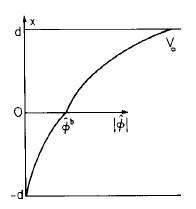
Fig. 5.15.2 Driven response

 

\[  \hat{\phi}(x) = \begin{cases} \hat{V}_o \frac{sinh(kx)}{sinh(kd)} - \hat{\phi}^b \frac{sinh \, k(x-d)}{sinh (kd)};  & x>0 \\\\ \hat{\phi}^b \frac{sinh \, k(x+d)}{sinh (kd)}  & x<0 \label{4}  \end{cases}  \]

The eigenfrequency equation is the denominator of Eq. 5.13.7 set equal to zero and evaluated with \(j \omega = s_n\):

\[ sinh (kd) + j \frac{2 \varepsilon_o}{k \sigma_s} (-j s_n - kU) cosh(kd) = 0 \label{5} \]

This expression has only one root,

\[ s_1 = jkU - \frac{k \sigma_s}{2 \varepsilon_o} tanh(kd) \label{6} \]

The one eigenfunction is determined by using the complex amplitudes of Sec. 5.13 with \(j \omega = s_1\) and \(\hat{V}_o = 0\).In this example, the eigenfunction has the distribution with \(x\) of Eq. \ref{4} with \(\hat{V}_o=0\), and a complex amplitude \(\hat{\phi}_1\) determined by the initial conditions:

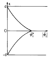
Fig. 5.15.3 Eigenfunction

\[  \hat{\phi}(x) = \begin{cases} \hat{\phi}_1^b \frac{sinh \, k(x-d)}{sinh (kd)};  & x>0 \\\\ \hat{\phi}_1^b \frac{sinh \, k(x+d)}{sinh (kd)}  & x<0 \label{7}  \end{cases}  \]

In general, the initial condition is on the charge distribution in the region \(-d < x < d\). In this example, the charge is confined to the sheet and only the one eigenmode is needed to meet the initial condition.

Suppose that when \(t = \theta\) there is no sheet charge and the excitation is suddenly turned on. The potential is given by Eq. \ref{1} with \(\hat{\phi}(x)\) and \(\hat{\phi}_1(x)\) given by Eqs. \ref{4} and \ref{7}. In terms of this potential, the surface charge is in general

\[ \sigma_f (z,t) = D_x^b - D_x^c = -\varepsilon_o k Re \Big \{ [ \frac{\hat{V}_o}{sinh (kd)} - 2 \hat{\phi}^b coth(kd)] e^{j (\omega t - kz)} - 2 \hat{\phi}_1^b coth(kd) e^{s_1 t - jkz} \Big \} \label{8} \]

To make of \(\sigma_f (z,0) = 0\), the eigenfunction amplitude must be such that when \(t = 0\), Eq. \ref{8} vanishes for all \(z\):

\[ \hat{\phi}_1^b = - \hat{\phi}^b + \frac{\hat{V}_o}{2 \, cosh(kd)} \label{9} \]

When \(t = 0^+\), the surface charge density is still zero, but the potential is finite over the entire region \(-d < x < d\). It can be shown by using Eq. \ref{9} in Eq. \ref{1} (evaluated when \(t = 0\) using Eqs. \ref{4} and \ref{7}) that at this instant the potential is what it would be in the absence of the conducting sheet.

The surface charge builds up at a rate determined by \(s_1\), which expresses the natural frequency as seen from a laboratory frame of reference. The oscillatory part is what is observed in the fixed frame as a spatially periodic distribution moves with the velocity of the material. If the driving voltage were suddenly turned off, the fields would decay in a way characterized by the same natural frequencies,with an oscillatory part reflecting the spatial periodicity of the initial charge distribution as it decays with a relaxation time \(2 \varepsilon_o / k \sigma_s\). Because the electric energy storage is in the free-space region, while the energy dissipation is within the sheet, this damping rate is not simply the bulk relaxation time of the conducting sheet.

In the long-wave limit, \(kd << 1\), the relaxation in this inhomogeneous system can be largely attributed to energy storage in the transverse electric field and dissipation due to the longitudinal electric field. On a scale of the system as a whole, the charge actually diffuses rather than relaxes. This can be seen by taking the limit \(kd << 1\) of Eq. \ref{6}:

\[ s_1 + (-jk)U = \frac{\sigma_s d}{2 \varepsilon_o} (-jk)^2 \label{10} \]

to obtain the dispersion equation for diffusion with convection. By infering time and \(z\) derivatives from the complex frequency \(s\) and \(-jk\) respectively, it can be seen from Eq. \ref{10} that in the long-wave limit the surface charge density is governed by the equation

\[ (\frac{\partial}{\partial{t}} + U \frac{\partial}{\partial{z}} \sigma_f = \frac{\sigma_s d}{2 \varepsilon_o} \frac{\partial{}^2 \sigma_f}{\partial{z^2}} \label{11} \]

This model is consistent with the distributed network shown in Fig. 5.15.4. The rigorous deduction of Eq. \ref{11} would exploit the space-rate expansion introduced in Sec. 4.12. The dominant electric fields are \(\overrightarrow{E} = E_x(z,t) \overrightarrow{i}_x \) in the air gaps and \(\overrightarrow{E} = E_z(z,t) \overrightarrow{i}_z \) in the sheet. This model is embedded in the discussion of the Van de Graaff machine given in Sec. 4.14, Eqs. 4.14.9 and 4.14.10.

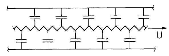
Fig. 5.15.4 Distributed network in the long-wave limit, equivalent to system of Fig. 5.13.1.

 

Heterogeneous Systems of Uniform Conductors

A generalization of the system of two uniformly con-ducting regions (the theme of Sec. 5.14) is shown in Fig. 5.15.5. Layers of material, each having the thickness \(d\), have different conductivities and move to the right with the velocity profile \(\overrightarrow{v} = U(x) \overrightarrow{i}_x\). Charge is confined to the interfaces, which have a negligible surface conductivity. Thus, the nth inter-face moves to the right with the velocity Un and is bounded from above and below by regions having the uniform properties \((\varepsilon_n, \sigma_n)\) and \((\varepsilon_n, \sigma_n)\) respectively. Variables evaluated just above and below the \(nth\) interface are denoted by \(n\) and \(n'\) respectively.

In the limit where the number of interfaces, \(N\), becomes large, the "stair-step" conductivity distribution approaches that of a continuous distribution. The following illustrates the second method of determining the natural frequencies, while giving insight as to why an infinite number of natural modes exists in systems having a distributed conductivity.

The regions just above and just below the \(nth\) interface are described by the planar transfer relations representing Laplace's equation, Eq. (a) of Table 2.16.1:

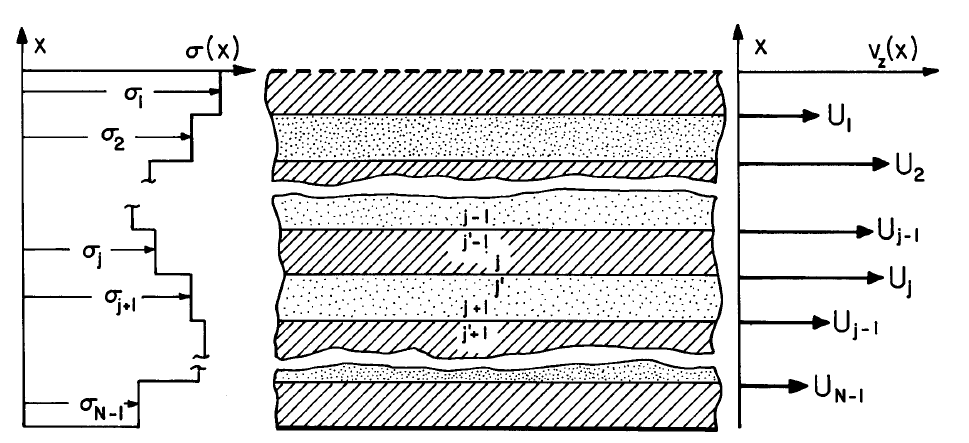
Fig. 5.15.5. A material having a conductivity that depends on x moves to the right with the velocity distribution \(v_x = U(x)\).

 

\[ \begin{bmatrix} \hat{D}_x^{n^{'}-1} \\  \hat{D}_x^{n} \end{bmatrix} = \varepsilon_n k \begin{bmatrix} -coth(kd) & \frac{1}{sinh(kd)} \\ -\frac{1}{sinh(kd)} & coth(kd) \end{bmatrix} \begin{bmatrix} \hat{\phi}^{n^{'}-1} \\  \hat{\phi}^{n} \end{bmatrix} \label{12}  \]

\[\begin{bmatrix} \hat{D}_x^{n^{'}} \\  \hat{D}_x^{n+1} \end{bmatrix} = \varepsilon_{n+1} k \begin{bmatrix} -coth(kd) & \frac{1}{sinh(kd)} \\ -\frac{1}{sinh(kd)} & coth(kd) \end{bmatrix} \begin{bmatrix} \hat{\phi}^{n^{'}} \\  \hat{\phi}^{n+1} \end{bmatrix} \label{13}  \]

At each interface, the potential is continuous:

\[ \hat{\phi}^{n^{'}-1} = \hat{\phi}^{n-1}; \, \hat{\phi}^{n^{'}} = \hat{\phi}^{n} \label{14} \]

With the understanding that the natural modes now identified are associated with the response to potential constraints at the transverse boundaries, potentials at the upper and lower surfaces must vanish:

\[ \hat{\phi}^o = 0; \, \hat{\phi}^{N+1} = 0 \label{15} \]

On the \(nth\) interface, conservation of charge (Eq. 5.12.4) requires the additional boundary condition:

\[ (-s + jkU_n) \hat{\sigma}_f^n = \frac{\sigma_n}{\varepsilon_n} \hat{D}_x^n - \frac{\sigma_{n+1}}{\varepsilon_{n+1}} \hat{D}_x^{n^{'}} \label{16} \]

At each interface, the surface charge is related to potentials at that and the adjacent interfaces, as can be seen by using Eqs. \ref{12} b, \ref{13} a and \ref{14} to write

\[ \hat{\sigma}_f^n = \hat{D}_x^n - \hat{D}_x^{n^{'}} = k \Big [ \frac{\varepsilon_n \hat{\phi}^{n-1}}{sinh(kd)} + (\varepsilon_n + \varepsilon_{n+1})coth(kd) \hat{\phi}^n - \frac{\varepsilon_{n+1} \hat{\phi}^{n+1}}{sinh(kd)} \Big ] \label{17} \]

This expression holds at each of the \(N\) interfaces. In view of the boundary conditions at the transverse boundaries, Eqs. \ref{15}, Eqs. \ref{17} are \(N\) equations for the \(N \sigma_f^{n^{'}}\) in terms of the interfacial potentials \(\hat{\phi}^n\):

\[ [\hat{\sigma}_f] = [A] \, [\hat{\phi}] \label{18} \]

where \([\hat{\sigma}_f]\) and \([\hat{\phi}]\) are \(Nth\) order column matrices and 

\[ [A] = \begin{bmatrix} k(\varepsilon_1 + \varepsilon_2) coth(kd) & -k \varepsilon_2 / sinh(kd) & 0 &  &  & \\  -k \varepsilon_2 / sinh(kd) & k(\varepsilon_2 + \varepsilon_3) coth(kd) & -k \varepsilon_3/ sinh(kd) & 0 & . & . & \\ 0 & & & & & \\ 0 & & & & & \\ . & & & 0 & -k\varepsilon_N / sinh(kd) & k (\varepsilon_N + \varepsilon_{N+1}) coth(kd) \\ . & & & & & &  \end{bmatrix}  \nonumber \]

Equation \ref{16} can similarly be written in terms of the potentials by using Eqs. \ref{12} b, \ref{13} a and \ref{14}:

\[ (-s + jkU_n) \hat{\sigma}_f^n = \frac{-k \sigma_n}{sinh(kd)} \hat{\phi}^{n-1} + k(\sigma_n \sigma_{n+1}) coth (kd) \hat{\phi}^n \frac{k \sigma_{n+1}}{sinh(kd)} \hat{\phi}^{n+1} \label{19} \]

In view of Eq. \ref{15}, this expression, written with \(n = 1,2,...,N,\) takes the matrix form

\[ \begin{bmatrix} -s+jkU_1 & 0 & 0 & \\  0 & -s + jkU_2 & 0 & \\ 0 & & &  \\ . & & & \\ . & & & -s + jk U_N \end{bmatrix} \begin{bmatrix} \hat{\sigma}_f^1 \\ \\ \\ \hat{\sigma}_f^N \end{bmatrix} = [B] [\hat{\phi}] \label{20} \]

where 

\[ [B] = \begin{bmatrix} k(\sigma_1 + \sigma_2) coth(kd) & \frac{-k \sigma_2}{sinh(kd)} & 0 & \\  \frac{-k \sigma_2}{sinh(kd)} & k(\sigma_2 + \sigma_3) coth(kd) & \frac{-k \sigma_3}{sinh(kd)} & 0 \\ 0 & & & 0\\ . & & & \\ . & 0 & \frac{-k \sigma_N}{sinh(kd)} & k (\sigma_N + \sigma_{N+1}) coth(kd) \end{bmatrix}  \nonumber \]

Now, if Eq. \ref{18} is inverted, so that = \([\hat{\phi} = [A]^-1 [\hat{\sigma}_f]\) and the column matrix \([\hat{\phi}]\) substituted on the right in Eq. \ref{20}, a set of equations are obtained which are homogeneous in the amplitudes \(\hat{\sigma}_f^n\),

\[ \begin{bmatrix} jkU_1-C_{11}-s & -C_{12} & -C_{13} & \\ -C_{21} & jkU_2 - C_{22} -s & -C_{23} & \\  &  &  &  \\ &  &  &  \\  &  &  &  \\ & & & jkU_N - C_{NN} -s \end{bmatrix} \begin{bmatrix} \hat{\sigma}_f^1 \\ \hat{\sigma}_f^2 \\ . \\  .  \\ . \\ \hat{\sigma}_f^N \end{bmatrix}  \label{21} \]

where \([C] = [B] \, [A]^{-1}\).

For the amplitudes to be finite, the determinant of the coefficients must vanish, and this constitutes the eigenfrequency equation \(D_1(s,k_x,k_y) = 0\). The determinant takes the standard matrix form for a characteristic value problem\(^1\). Expanded, it is an \(Nth\) order polynomial in \(s\), and hence has \(N\) roots which are the natural frequencies.

As an example, suppose that there is a single interface, \(N=1\). Then, from Eqs. \ref{18} and \ref{20},

\[ A^{-1} = \frac{1}{k (\varepsilon_1 + \varepsilon_2) coth(kd)} ; \, B = k(\sigma_1 + \sigma_2) coth(kd) \label{22} \]

and it follows that \(C_{11} - (\sigma_1 + \sigma_2)/(\varepsilon_1+ \varepsilon_2)\) so that Eq. \ref{21} gives the single eigenfrequency

\[ s_1 = jkU_1 - \Big (\frac{ \sigma_1 + \sigma_2}{\varepsilon_1 + \varepsilon_2} \Big ) \label{23} \]

With \(a = b = d\), this result is consistent with setting the denominator of Eq. 5.14.8 equal to zero and solving for \(j\omega).

With two interfaces, there are two eigenmodes, with frequencies determined from Eq. \ref{21}:

\[  \begin{bmatrix} (jkU_1 - C_{11} -s) & -C_{12} \\ -C_{21} & (jkU_2 - C_{22} -a) \end{bmatrix} = 0 \label{24} \]

The entries \(C_{ij}\) follow from \([C] = [B] \, [A]^{-1} \)

\[ [C] = \begin{bmatrix} k(\sigma_1 + \sigma_2) coth(kd) & \frac{-k \sigma_2}{sinh(kd)} \\  \frac{-k \sigma_2}{sinh(kd)} & k (\sigma_2 + \sigma_3) coth(kd) \end{bmatrix} \begin{bmatrix} \frac{k(\varepsilon_2 + \varepsilon_3) coth(kd)}{DET} & \frac{k \varepsilon_2}{DET \, sinh(kd)} \\  \frac{k \varepsilon_2}{DET \, sinh(kd)} & \frac{k(\varepsilon_1 + \varepsilon_2) coth(kd)}{DET} \end{bmatrix} \\ = \frac{k^2}{DET} \begin{bmatrix} [(\sigma_1 + \sigma_2)(\varepsilon_2 + \varepsilon_3) coth^2 (kd) - \frac{\varepsilon_2 \sigma_2}{sinh^2  (kd)} ] & [ ( \sigma_1 \varepsilon_2 - \sigma_2 \varepsilon_1) \, \frac{coth(kd)}{sinh(kd)}] \\ [ (\sigma_3 \varepsilon_2 - \sigma_2 \varepsilon_3) \, \frac{coth(kd)}{sinh(kd)}] & [ ( \sigma_2 + \sigma_3)(\varepsilon_1 + \varepsilon_2) coth^2 (kd) - \frac{\sigma_2 \varepsilon_2}{sinh^2 (kd)}] \end{bmatrix} \label{25} \]

where 

\[ DET \equiv k^2 [ (\varepsilon_1 + \varepsilon_2) (\varepsilon_2 + \varepsilon_3) coth^2 (kd) - \varepsilon_2^2/sinh^2 (kd)] \nonumber \]

The eigenfrequency equation, Eq.\ref{24}, is quadratic in \(s\), and can be solved to obtain the two eigenfrequencies

\[ \begin{pmatrix} s_1 \\ s_2 \end{pmatrix} = \frac{1}{2} [jk(U_1 + U_2) - C_{11} - C_{22}] \pm \sqrt{\frac{1}{4} [ jk (U_1 + U_2) - C_{11} - C_{22}]^2 - (jkU_1 - C_11)(jkU_2 - C_{22}) - C_{12} C_{21}} \label{26} \]

where the \(C_{ij}\) are given by Eq. \ref{25} \nonumber \]

The \(N\) eigenmodes can be used to represent the temporal transient resulting from turning on or turning off a spatially periodic drive. Although more complicated, the procedure is in principle much as illustrated in the sheet conductor example. As expressed by Eq. \ref{1}, the transient is in general a superposition of the driven response (for the turn on) and the natural modes. The \(N\) eigenmodes make it possible to satisfy \ref{N} initial conditions specifying the surface charges on the \(N\) interfaces.

In the limit where \(N\) becomes infinite, the number of modes becomes infinite and the physical system is one having a smooth distribution of conductivity \(\sigma(x)\), and permittivity, \(\varepsilon(x)\). This infinite set of internal modes can also be used to account for initial conditions. Such modes are encountered again in Sec. 6.10, in connection with magnetic diffusion, where an infinite number of modes are possible even with systems having uniform properties. What has been touched on here is the behavior ofsmoothly inhomogeneous systems, described by linear differential equations with space-varying coefficients. The finite mode model, implicit to approximating \(\sigma(x)\) and \(\varepsilon(x)\) by the stair-step distribution is one way to take into account the terms \(\overrightarrow{E} \cdot \nabla \sigma\) and \(\overrightarrow{E} \cdot \nabla \varepsilon\) in the charge relaxation law, Eq. 5.10.6.

---

1. F. E. Hohn, Elementary Matrix Algebra, 2nd ed., Macmillan Company, New York, 1964, p. 273.