
11.4: Mass Spring Example
- Page ID
- 19007

Examples in this section and the next section will illustrate how we can use the Euler-Lagrange equation to find the equation of motion describing an energy conversion process. Consider a system comprised of a mass and a spring where energy is transfered between spring potential energy stored in the compressed spring and kinetic energy of the mass. The mass is specified by \(m\) in kg. It is attached to a spring with spring constant \(K\) in \(\frac{J}{m^2}\). The position of the mass is specified by \(x(t)\) where \(x\) is the dependent variable in meters and \(t\) is the independent variable time in seconds. Assume this mass and spring are either fixed on a level plane or in some other way not influenced by gravity. This mass spring system is illustrated on the left side of Fig. \(\PageIndex{1}\). When the spring is compressed, the system gains spring potential energy. When the spring is released, energy is converted from spring potential energy to kinetic energy. Assume no other energy conversion processes, such as heating due to friction, occur.
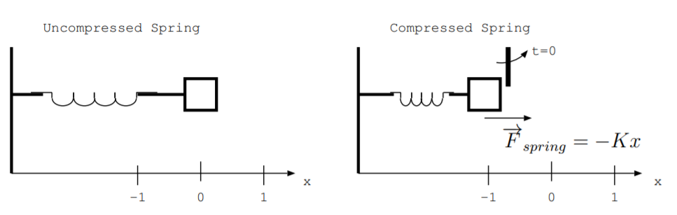
The right side of Fig. \(\PageIndex{1}\) shows the compressed spring held in place by a restraint. For \(t < 0\), the system has no kinetic energy because the mass is not moving, and the system has potential energy in the compressed spring. At this time, the mass is at position \(x\) where \(x < 0\). The spring exerts a force on the mass,
\[\overrightarrow{F}_{spring}=-K x \hat{a}_{x} \nonumber \]
which is in the \(\hat{a}_{x}\) direction.
At \(t = 0\), the restraint is removed, and the spring potential energy is converted to kinetic energy. The first form is spring potential energy.
\[E_{potential\,energy} = \frac{1}{2}Kx^2 \nonumber \]
The second form is kinetic energy of the mass.
\[E_{kinetic} = \frac{1}{2} m \left( \frac{dx}{dt} \right)^2 \nonumber \]
At any instant of time, when the mass is at location \(x(t)\), the total energy is represented by the Hamiltonian.
\[H = E_{total} = E_{potential\,energy} + E_{kinetic} \nonumber \]
\[H=\frac{1}{2} K x^{2}+\frac{1}{2} m\left(\frac{d x}{d t}\right)^{2} \label{11.4.5} \]
The Lagrangian represents the difference between the forms of energy.
\[\mathcal{L}=E_{potential\,energy} -E_{kinetic} \nonumber \]
\[\mathcal{L}\left(t, x, \frac{d x}{d t}\right)=\frac{1}{2} K x^{2}-\frac{1}{2} m\left(\frac{d x}{d t}\right)^{2} \nonumber \]
Both the Hamiltonian and Lagrangian have units of joules. The generalized potential is
\[\frac{\partial \mathcal{L}}{\partial x} = Kx \nonumber \]
in units of newtons. Note that \(Kx = − \overrightarrow{F}_{spring}\). The generalized momentum is
\[\mathbb{M}=\frac{\partial \mathcal{L}}{\partial\left(\frac{d x}{d t}\right)}=-m \frac{d x}{d t} \nonumber \]
in units of \(\frac{kg \cdot m}{s}\) which is the units of momentum.
At \(t = 0\), the restraint is removed. The mass follows the path \(x(t)\). If we know the Lagrangian, we can find the path by trial and error. To find the path in this way, guess a path \(x(t)\) that the mass follows and calculate the action.
\[\mathbb{S}=\left|\int_{t_{1}}^{t_{2}} \frac{1}{2} m\left(\frac{d x}{d t}\right)^{2}-\frac{1}{2} K x^{2}\right| d t \label{11.4.10} \]
Repeatedly guess another path, and calculate the action. The path with the least action of all possible paths is the path that the mass follows. This path has the smallest difference between the potential energy and the kinetic energy integrated over time.
We can think of many possible, but not physical, paths \(x(t)\) that the mass can follow. Figure \(\PageIndex{2}\) illustrates two nonphysical paths as well as the physical path derived below. Paths are considered over the time interval \(0 < t < 1\). All three paths assume that initially, at \(t = 0\), the spring is compressed so that the mass is at location \(x(0) = -1\). Also, they assume that at the end of the interval, at \(t = 1\), the spring has expanded so that the mass is at location \(x(1) = 1\). The possible paths illustrated in the figure are
\[x_{1}(t)=2 t-1 \quad(\text { not physical })\nonumber \]
\[x_{2}(t)=2 t^{2}-1 \quad(\text { not physical })\nonumber \]
and
\[x_{3}(t)=-\cos (\pi t) \quad(\text { physical })\nonumber \]
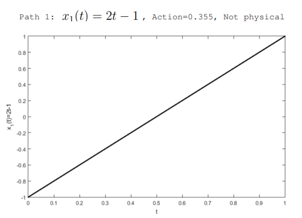
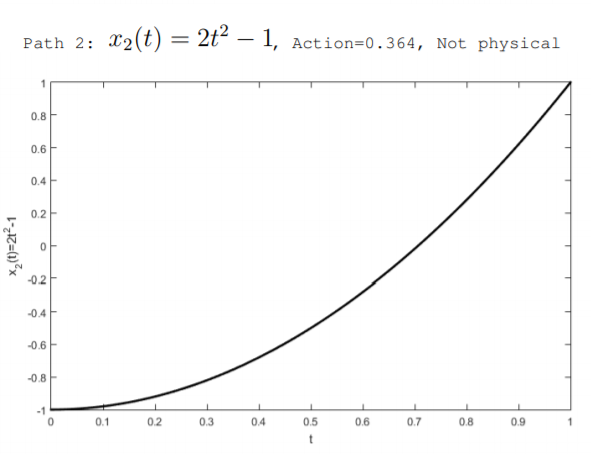
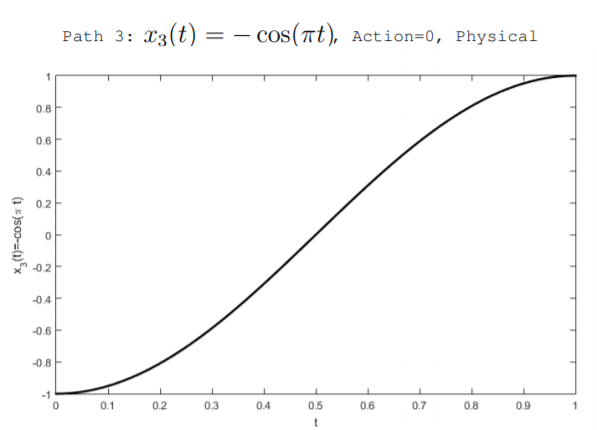
The path \(x_1(t)\) describes a case where the mass travels at a constant speed. The path \(x_2(t)\) describes a case where the mass accelerates when the restraint is removed, and the path \(x_3(t)\) describes a case where the mass first accelerates then slows. The action of each path can be calculated using Equation \ref{11.4.10}. For example purposes, the values of \(m = 1 kg\) and \(K = \pi^2 \frac{J}{m^2}\) are used. The path \(x_1(t)\) has \(\mathbb{S} = 0.355\), the path \(x_2(t)\) has \(\mathbb{S} = 0.364\), and the physical path \(x_3(t)\) has zero action \(\mathbb{S} = 0\). We can derive the path that minimizes the action and that is found in nature using the Euler-Lagrange equation.
\[\frac{\partial \mathcal{L}}{\partial x}-\frac{d}{d t} \frac{\partial \mathcal{L}}{\partial\left(\frac{d x}{d t}\right)}=0 \nonumber \]
The first term is the generalized potential. The second term is the time derivative of the generalized momentum. The equation of motion is found by putting these pieces together.
\[Kx+m\frac{d^2x}{dt^2} = 0 \label{11.4.12} \]
The first term of the equation of motion is \(- \left| \overrightarrow{F}_{spring} \right|\). The second term represents the acceleration of the mass. We have just found the equation of motion, and it is a statement of Newton's second law, force is mass times acceleration. It is also a statement of conservation of force on the mass.
Equation \ref{11.4.12} is a second order linear differential equation with constant coefficients. It is the famous wave equation, and its solution is well known
\[x(t)=c_{0} \cos \left(\sqrt{\frac{K}{m}} t\right)+c_{1} \sin \left(\sqrt{\frac{K}{m}} t\right) \nonumber \]
where \(c_0\) and \(c_1\) are constants determined by the initial conditions. If we securely attach the mass to the spring, as opposed to letting the mass get kicked away, it will oscillate as described by the path \(x(t)\). Energy is conserved in this system. To verify conservation of energy, we can show that the total energy does not vary with time. The total energy is given by the Hamiltonian of Equation \ref{11.4.5}. In this example, both the Hamiltonian and the Lagrangian do not explicitly depend on time, \(\frac{\partial H}{\partial t} =0\) and \(\frac{\partial \mathcal{L}}{\partial t} = 0\). Instead, they only depend on changes in time. For this reason, we say both the total energy and the Lagrangian have time translation symmetry, or we say they are time invariant. The spring and mass behave the same today, a week from today, and a year from today.
We can also verify conservation of energy algebraically by showing that \(\frac{dH}{dt} = 0\).
\[\frac{d H}{d t}=\frac{\partial H}{\partial t}+\frac{\partial H}{\partial x} \frac{d x}{d t}+\frac{\partial H}{\partial\left(\frac{d x}{d t}\right)} \frac{d^{2} x}{d t^{2}} \nonumber \]
\[\frac{d H}{d t}=0+K x \frac{d x}{d t}+m \frac{d x}{d t} \frac{d^{2} x}{d t^{2}} \nonumber \]
\[\frac{d H}{d t}=\frac{d x}{d t}\left(K x+m \frac{d^{2} x}{d t^{2}}\right)=0 \nonumber \]
Notice that the quantity in parentheses in the line above must be zero from the equation of motion. The Euler-Lagrange equation can be split into a pair of first order differential equations called Hamilton's equations.
\[\frac{d \mathbb{M}}{d t} =-\frac{\partial H}{\partial x} \quad \text { and } \frac{d x}{d t} =\frac{\partial H}{\partial \mathbb{M}} \nonumber \]
This example is summarized in Table \(\PageIndex{1}\). In analogy to language used to describe circuits and electromagnetics, the relationship between the generalized path and the generalized potential is referred to as the constitutive relationship. Following Equation 11.1.6, the ratio of the generalized path to generalized potential is the generalized capacity, and in this example, it is the inverse of the spring constant. While displacement \(x\) is assumed to be scalar, the vector \(\overrightarrow{x}\) is used in the table for generality.
| Energy storage device | Linear spring |
|---|---|
| Generalized Path | Displacement \(\overrightarrow{x}\) in m |
| Generalized Potential | \(\overrightarrow{F}\) Force in \(\frac{J}{m} = N\) |
| Generalized Capacity | \(\frac{1}{K}\) in \(\frac{m^2}{J}\) |
| Constitutive relationship | \(\overrightarrow{x} = \frac{1}{K}\overrightarrow{F}\) |
| Energy | \(\frac{1}{2}\frac{1}{K}|\overrightarrow{x}|^2 = \frac{1}{2}K|\overrightarrow{F}|^2\) |
| Law for potential | Newton's Second Law \(\overrightarrow{F} = m\overrightarrow{a}\) |