13.3: Derivation of the Lagrangian

The purpose of this chapter is to find the voltage \(V (r)\) and the charge density \(\rho_{ch}(r)\) around an atom, and we will use calculus of variations to accomplish this task. We need to make some rather severe assumptions to make this problem manageable. Consider an isolated neutral atom with many electrons around it. Assume \(T \approx 0\) K, so all electrons occupy the lowest possible energy levels. Assume the atom is spherically symmetric. All of the quantities we encounter, such as voltage, charge density, and Lagrangian, vary with \(r\) but do not vary with \(\theta\) or \(\phi\). We will use spherical coordinates with the origin at the nucleus of the atom. While quantities vary with position, assume no quantities vary with time. The charge density \(\rho_{ch}(r)\) tells us where the electrons are most likely on average to be found. It is related to the quantum mechanical wave function, \(\psi\), by

\[\rho_{c h}=-q \cdot|\psi|^{2} \nonumber \]

where \(q\) is the magnitude of the charge of an electron. Assume that all of the electrons surrounding the atom are distributed uniformly and can be treated as if they were a uniform electron cloud of some charge density.

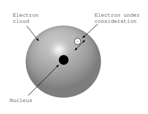
Pick one of the electrons of the atom, and consider what happens when the electron is moved radially in and out. Figure \(\PageIndex{1}\) illustrates this situation. As the electron moves, energy conversion occurs. The goal of this section is to write down the Hamiltonian and Lagrangian for this energy conversion process. We write these quantities in the units of energy per unit volume per valence electron under consideration.

Figure \(\PageIndex{1}\): Illustration of an atom.

To understand what happens when the electron is moved, consider the energy of the atom in more detail. Coulomb's law, introduced in Equation 1.6.2, tells us that charged objects exert forces on other charged objects. More specifically, the electric field intensity \(\overrightarrow{E}\) due to a point charge of \(Q\) coulombs a distance \(r\) away surrounded by a material with permittivity \(\epsilon\) is given by

\[\overrightarrow{E}=\frac{Q \hat{a}_{r}}{4 \pi \epsilon r^{2}}. \nonumber \]

The atom is composed of \(N\) positively charged protons. The electron under consideration feels an attractive Coulomb force due to these protons. Additionally, the atom has \(N\) electrons, and \(N - 1\) of these exert a repulsive Coulomb force on the electron under consideration. Since a charge separation and electric field exist, energy is stored. Call the component of the energy of the atom due to the Coulomb interaction between the protons of the nucleus and the electron under consideration \(E_{Coulomb\, e \,nucl}\). Call the Coulomb interaction between the electron under consideration and all other electrons \(E_{e\, e \,interact}\). The atom also has kinetic energy. Call the kinetic energy of the nucleus \(E_{kinetic\, nucl}\) and the kinetic energy of all of the electrons \(E_{kinetic\, e}\). The energy of the atom is the sum of all of these terms.

\[E_{atom} = E_{Coulomb\, e \,nucl.} + E_{kinetic\, nucl} + E_{e\, e \,interact} + E_{kinetic \,e} \nonumber \]

Energy due to spin of the electrons and protons is ignored as is energy due to interaction with any other nearby charged objects. At \(T \approx 0\) K, the kinetic energy of the nucleus will be close to zero, so we can ignore the term, \(E_{kinetic\, nucl} \approx 0\). The quantity \(E_{kinetic\, e}\) cannot be exactly zero. In Chapter 6 we plotted energy level diagrams for electrons around an atom. Even at \(T = 0\) K, electrons have some internal energy, and this energy is denoted by the energy level occupied.

If we have a large atom with many electrons around it, the Coulomb interaction between any one electron and the nucleus is shielded by the Coulomb interaction from all other electrons. More specifically, suppose we have an isolated atom with \(N\) protons in the nucleus and \(N\) electrons around it. If we pick one of the electrons, \(E_{Coulomb\, e \,nucl}\) for that electron describes the energy stored in the electric field due to the charge separation between the nucleus of positive charge \(Nq\) and that electron. However, there are also \(N - 1\) other electrons which have a negative charge. The term \(E_{e\, e \,interact}\) describes the energy stored in the electric field due to the charge separation between the \(N - 1\) other electrons and the electron under consideration. These terms somewhat cancel each other out because the electron under consideration interacts with \(N\) protons each of positive charge q and \(N - 1\) electrons each of negative charge \(-q\). However, the terms do not go away completely. Calculating

\[E_{Coulomb\, e \,nucl} + E_{e\, e \,interact} \nonumber \]

is complicated because the electrons are in motion, and we do not really know where they are or even where they are most likely to be found. In fact, we are trying to solve for where they are likely to be found.

As we move the electron under consideration in and out radially, energy is transferred between (\(E_{Coulomb\, e \,nucl} + E_{e\, e \,interact}\)) and \(E_{kinetic\, e}\). The Hamiltonian is the sum of these two forms of energy per unit volume, and the Lagrangian is the difference of these two forms of energy per unit volume. Both quantities have the units \(\frac{J}{m^3}\). Choose voltage \(V (r)\) as the generalized path and charge density \(\rho_{ch}(r)\) as the generalized potential. The independent variable of these quantities is radial position \(r\), not time. We can now write the Hamiltonian and Lagrangian.

\[H\left(r, V, \frac{d V}{d r}\right) = \left(\frac{E_{Coulomb\, e \,nucl}}{\mathbb{V}} + \frac{E_{e\, e \,interact}}{\mathbb{V}}\right) + \frac{E_{kinetic\, e}}{\mathbb{V}} \nonumber \]

\[\mathcal{L} \left(r, V, \frac{d V}{d r}\right) = \left(\frac{E_{Coulomb\, e \,nucl}}{\mathbb{V}} + \frac{E_{e\, e \,interact}}{\mathbb{V}}\right) - \frac{E_{kinetic\, e}}{\mathbb{V}} \nonumber \]

The next step is to write

\[\frac{E_{Coulomb\, e \,nucl}}{\mathbb{V}} + \frac{E_{e\, e \,interact}}{\mathbb{V}} \nonumber \]

in terms of the path \(V\). As detailed in Table 12.2.3, the energy density due to an electric field \(\overrightarrow{E}\) is given by

\[\frac{E}{\mathbb{V}} = \frac{1}{2}\epsilon |\overrightarrow{E}|^2. \nonumber \]

Remember that \(E\) represents energy while \(\overrightarrow{E}\) represents electric field. Electric field is the negative gradient of the voltage \(V (r)\).

\[\overrightarrow{E} = -\overrightarrow{\nabla}V. \nonumber \]

We can combine these expressions and Equation 13.2.6 to write the first term of the Hamiltonian and the Lagrangian in terms of the generalized path.

\[\frac{E_{Coulomb\, e \,nucl}}{\mathbb{V}} + \frac{E_{e\, e \,interact}}{\mathbb{V}} = \frac{1}{2}\epsilon |\overrightarrow{\nabla}V|^2 \nonumber \]

\[H\left(r, V, \frac{d V}{d r}\right) = \left(\frac{1}{2}\epsilon |\overrightarrow{\nabla}V|^2\right) + \frac{E_{kinetic\, e}}{\mathbb{V}} \nonumber \]

\[\mathcal{L} \left(r, V, \frac{d V}{d r}\right) = \left(\frac{1}{2}\epsilon |\overrightarrow{\nabla}V|^2\right) - \frac{E_{kinetic\, e}}{\mathbb{V}} \nonumber \]

The next task is to describe the remaining term \(\frac{E_{kinetic\, e}}{\mathbb{V}}\) as a function of the generalized path too. This task is a bit more challenging. We continue to take the approach of making severe approximations until it is manageable. We need to express \(\rho_{ch}(r)\) as a function of \(V (r)\). Then with some algebra, \(\frac{E_{kinetic\, e}}{\mathbb{V}}\) can be written purely as a function of \(V (r)\).

We want to generalize about the kinetic energy of the electrons. However, each electron has its own velocity \(\overrightarrow{v}\) and momentum \(\overrightarrow{M}\). These quantities depend on position

\[\overrightarrow{r} = r \hat{a}_r + \theta \hat{a}_{\theta} + \phi \hat{a}_{\phi} \nonumber \]

in some unknown way. Furthermore, the calculation of \(\frac{E_{kinetic\, e}}{\mathbb{V}}\) depends on charge density \(\rho_{ch}(r)\), which is the unknown quantity we are trying to find. We have more luck by describing these quantities in reciprocal space, introduced in Sec. 6.3. Position is denoted in reciprocal space by a wave vector

\[\overrightarrow{k} = \tilde r \hat{a}_r + \tilde \theta \hat{a}_{\theta} + \tilde \phi \hat{a}_{\phi} \label{13.3.14} \]

We can describe the properties of a material by describing how they vary with position in real space. For example, \(\rho_{ch}(r)\) represents the charge density of electrons as a function of distance r from the center of the atom. We may be interested in how other quantities, such as the energy required to rip off an electron or the kinetic energy internal to an electron, vary with position in real space too. Instead of describing how quantities vary with position in real space, we can describe how quantities vary with spatial frequency of electrons. This is the idea behind representing quantities in reciprocal space. We may be interested in how the charge density of electrons varies as a function of the spatial frequency of charges in a crystal or other material, and this is the idea represented by functions of wave vector such as \(\rho_{ch}(\overrightarrow{k})\). We are trying to solve for charge density \(\rho_{ch}(r)\). We expect that electrons are more likely to be found at certain distances \(r\) from the center of the atom than at other distances. However, there is no pattern to the charge density as a function of wave vector, \(\rho_{ch}(\overrightarrow{k})\). Assume that \(\rho_{ch}\) is roughly constant with respect to \(|\overrightarrow{k}|\) up to some level. With some more work, this assumption will allow us to solve for charge density \(\rho_{ch}(r)\).

The kinetic energy of a single electron is given by

\[\frac{E_{kinetic\, e}}{e^-} = \frac{1}{2}m|\overrightarrow{v}|^2 \nonumber \]

where \(m\) is the mass of the electron. We can write this energy in terms of momentum, \(\overrightarrow{M} = m\overrightarrow{v}\). (Note that momentum \(\overrightarrow{M}\) and generalized momentum \(\mathbb{M}\) are different and have different units.)

\[\frac{E_{kinetic\, e}}{e^-} = \frac{|\overrightarrow{M}|^2}{2m} \nonumber \]

We do not know how the energy varies as a function of position r. Instead, we can write the energy as a function of the crystal momentum \(\overrightarrow{M}_{crystal}\) or the wave vector \(\overrightarrow{k}\), and we know something about the variation of these quantities. Crystal momentum is equal to the wave vector scaled by the Planck constant.

\[\overrightarrow{M}_{crystal} = \hbar \overrightarrow{k} \nonumber \]

It has the units of momentum \(\frac{kg \cdot m}{s}\), and it was introduced in Sec. 6.3.2. The kinetic energy of one electron as a function of the crystal momentum is given by

\[\frac{E_{kinetic\, e}}{e^-} = \frac{\left(\overrightarrow{M}_{crystal}\right)^2}{2m} = \frac{\left(\hbar |\overrightarrow{k}|\right)^2}{2m}. \label{13.3.18} \]

A vector in reciprocal space is represented Equation \ref{13.3.14}, and Equation \ref{13.3.18} can be simplified because we are assuming spherical symmetry \(\tilde \theta = \tilde \phi = 0\). The magnitude of the wave vector becomes \(|\overrightarrow{k}| = \tilde r\), and we can write the energy as

\[\frac{E_{kinetic\, e}}{e^-} = \frac{\hbar^2 \tilde r^2}{2m}. \label{13.3.19} \]

Just as each electron has its own momentum \(m|\overrightarrow{v}|\), each electron has its own crystal momentum \(\hbar |\overrightarrow{k}|\). However, we know some information about the wave vector \(|\overrightarrow{k}|\) of the electrons in the atom. At \(T = 0\) K, electrons occupy the lowest allowed energy states. Energy states are occupied up to some highest occupied state called the Fermi energy \(E_f\). While electrical engineers use the term Fermi energy, chemists sometimes use the term chemical potential \(\mu_{chem}\). The lowest energy states, are occupied while the higher ones are empty. Similarly, wave vectors are occupied up to some highest occupied wave vector called the Fermi wave vector \(k_f\).

\[ |\overrightarrow{k}| = \begin{cases} \text{filled state} & \tilde r < k_f \\ \text{empty state} & \tilde r > k_f \end{cases} \nonumber \]

The Fermi energy and the Fermi wave vector are related by

\[E_f = \frac{\hbar^2 k^2_f}{2m}. \label{13.3.21} \]

We use the idea of reciprocal space to write an expression for the kinetic energy of the electrons per unit volume [136, p. 49]. The kinetic energy due to any one electron as a function of position in reciprocal space is given by Equation \ref{13.3.19}. Note that at each value of \(|\overrightarrow{k}| = \tilde r\), the electron has a different kinetic energy. To find the kinetic energy per unit volume due to all electrons, we integrate over all \(|\overrightarrow{k}| = \tilde r\) in spherical coordinates that are occupied by electrons, and then we divide by the volume occupied in \(\overrightarrow{k}\) space.

\[\frac{E_{kinetic\, e}}{\mathbb{V}} = \frac{1}{\text{vol. occupied in } k \text{ space}} \cdot \int_{\text{filled } k \text{ levels}} \left(\frac{E_{kinetic\, e}}{e^-}\right)\left(\frac{e^-}{\text{volume}}\right) d (\text{vol. all } k \text{ space}) \nonumber \]

The number of electrons per unit volume is given by

\[\left(\frac{e^-}{\text{volume}}\right) = \frac{-\rho_{ch}}{q}. \nonumber \]

The volume occupied in reciprocal space is \(\frac{4}{3}\pi k^3_f\), the volume of a sphere of radius \(k_f\).

\[\frac{E_{kinetic\, e}}{\mathbb{V}} = \frac{1}{\frac{4}{3}\pi k^3_f} \cdot \int_{\text{filled } k \text{ levels}} \left(\frac{\hbar^2 \tilde r^2}{2m}\right)\left(\frac{-\rho_{ch}}{q}\right) d (\text{vol. all } k \text{ space}) \nonumber \]

A differential element of the volume is expressed as

\[d^3 |\overrightarrow{k}| = \tilde r^2 \sin \tilde \theta\, d \tilde r \,d \tilde \theta \,d \tilde \phi. \nonumber \]

\[\frac{E_{kinetic\, e}}{\mathbb{V}} = \frac{1}{\frac{4}{3}\pi k^3_f} \cdot \int_{\text{filled } k \text{ levels}} \left(\frac{\hbar^2 |\overrightarrow{k}|^2}{2m}\right)\left(\frac{-\rho_{ch}}{q}\right) (\tilde r^2 \sin \tilde \theta\, d \tilde r \,d \tilde \theta \,d \tilde \phi) \nonumber \]

As described above, electrons occupy states in reciprocal space only with \(0 \leq \tilde r \leq k_f\).

\[\frac{E_{kinetic\, e}}{\mathbb{V}} = \frac{1}{\frac{4}{3}\pi k^3_f} \cdot \int\limits_{\tilde r = 0}^{k_f} \,\int\limits_{\tilde \theta = 0}^{\pi} \,\int\limits_{\tilde \phi = 0}^{2\pi} \left(\frac{\hbar^2 \tilde r^2}{2m}\right)\left(\frac{-\rho_{ch}}{q}\right) (\tilde r^2 \sin \tilde \theta\, d \tilde r \,d \tilde \theta \,d \tilde \phi) \nonumber \]

The integral above can be evaluated directly. The first step to evaluate it is to pull constants outside. As described above, \(\rho_{ch}\) varies with \(r\) but not \(\tilde r\), so it can be pulled outside the integral too.

\[\frac{E_{kinetic\, e}}{\mathbb{V}} = \frac{-1}{\frac{4}{3}\pi k^3_f} \cdot \frac{\hbar^2 \rho_{ch}}{2mq} \int\limits_{\tilde r = 0}^{k_f} \,\int\limits_{\tilde \theta = 0}^{\pi} \,\int\limits_{\tilde \phi = 0}^{2\pi} \tilde r^4 \sin \tilde \theta\, d \tilde r \,d \tilde \theta \,d \tilde \phi \nonumber \]

The integral separates and can be evaluated.

\[\frac{E_{kinetic\, e}}{\mathbb{V}} = \frac{-1}{\frac{4}{3}\pi k^3_f} \cdot \frac{\hbar^2 \rho_{ch}}{2mq} \left( \int\limits_{\tilde \theta = 0}^{\pi} \,\int\limits_{\tilde \phi = 0}^{2\pi} \sin \tilde \theta\, d \tilde r \,d \tilde \theta \,d \tilde \phi \right) \left( \int\limits_{\tilde r = 0}^{k_f} \tilde r^4 d \tilde r \right) \nonumber \]

\[\frac{E_{kinetic \, e}}{\mathbb{V}} = \frac{-1}{\frac{4}{3} \pi k^3_f} \cdot \frac{\hbar^2 \rho_{ch}}{2mq}4\pi \left(\frac{{k_f}^5}{5}\right) \nonumber \]

\[\frac{E_{kinetic \, e}}{\mathbb{V}} =\frac{-3 \rho_{ch} k^2_f \hbar^2}{10mq} \label{13.3.31} \]

Charge density is a function of position in real space \(r\), and we are in the process of solving for this function, \(\rho_{ch}(r)\). However, it also depends on the Fermi energy \(E_f\), and hence Fermi wave vector \(k_f\), for the atom. Next, we find the relationship between \(\rho_{ch}\) and \(k_f\). Two electrons are allowed per energy level (spin up and spin down), hence per filled \(k\) state. The number of filled states per atom in reciprocal space is related to the charge density.

\[\rho_{ch} = -2q \left( \frac{\text{no. filled } k \text{ states}}{\text{unit vol. in } k \text{ space}}\right) \nonumber \]

In Sec. 6.3.1, we saw that a primitive cell in reciprocal space was \((2 \pi )^3\) times the primitive cell in real space, so

\[(\text{unit vol. } k \text{ space}) = (2 \pi )^3 \cdot (\text{unit vol. real space}) = (2 \pi )^3. \nonumber \]

We know something about the wave vectors of filled states in reciprocal space. At \(T = 0\) K, the lowest states are filled, and all others are empty, and they are filled up to a radius of \(k_f\). The volume of a sphere of radius \(k_f\) is given by \(\frac{4}{3}\pi k^3_f\), and this represents the number of filled \(k\) states per volume of reciprocal space. We can therefore simplify the expression above.

\[\rho_{ch} = -2q \cdot \frac{4}{3} \pi k_f^3 \cdot \frac{1}{(2 \pi )^3} \nonumber \]

\[\rho_{ch} = \frac{-q}{3 \pi^2}k_f^3 \nonumber \]

\[k_f = \left(\frac{-3 \pi^2}{q}\rho_{ch}\right)^{1/3} \label{13.3.36} \]

We want to write \(\frac{E_{kinetic\, e}}{\mathbb{V}}\) as a function of generalized path \(V\). We can now achieve this task by combining Equations \ref{13.3.31} and \ref{13.3.36}.

\[\frac{E_{kinetic \, e}}{\mathbb{V}}= \frac{-3\hbar^2}{10mq}\rho_{ch} \left(\frac{-3\pi^2}{q}\rho_{ch}\right)^{2/3} \nonumber \]

\[\frac{E_{kinetic \, e}}{\mathbb{V}}= \frac{-3\hbar^2}{10mq} \left(\frac{-3\pi^2}{q}\right)^{2/3} \rho_{ch}^{5/3} \nonumber \]

Electrical energy is the product of charge and voltage. More specifically, from Equation 2.2.7, it is given by

\[E = \frac{1}{2}QV. \nonumber \]

Electrical energy density is then given by

\[\frac{E}{\mathbb{V}} = \frac{1}{2}\rho_{ch}V. \label{13.3.40} \]

Use Equation \ref{13.3.40} to relate \(\rho_{ch}\) and \(V\).

\[\frac{E_{kinetic \, e}}{\mathbb{V}}= \frac{1}{2}\rho_{ch}V =\frac{-3\hbar^2}{10mq} \left(\frac{-3\pi^2}{q}\right)^{2/3} \rho_{ch}^{5/3} \nonumber \]

We have now related the generalized path and the generalized potential.

\[V = \frac{-3\hbar^2}{5mq} \left(\frac{-3\pi^2}{q}\right)^{2/3} \rho_{ch}^{2/3} \nonumber \]

\[\rho_{ch} = \left(\frac{-5mq}{3\hbar^2} \cdot \left(\frac{-3\pi^2}{q}\right)^{-2/3} \right)^{3/2} V^{3/2} \nonumber \]

\[\rho_{ch} = \left[ \left(\frac{-5mq}{3\hbar^2}\right)^{3/2} \left(\frac{-q}{3\pi^2}\right)\right] \cdot V^{3/2} \nonumber \]

Finally, we can write \(\frac{E_{kinetic\, e}}{\mathbb{V}}\) as a function of \(V\).

\[\frac{E_{kinetic \, e}}{\mathbb{V}}= \left[ \left(\frac{-5mq}{3\hbar^2}\right)^{3/2} \left(\frac{-q}{3\pi^2}\right)\right]V^{5/2} \nonumber \]

Notice that the quantity in brackets above is constant. The coefficient \(c_0\) is defined from the term in brackets.

\[c_0 = \left(\frac{-5mq}{3\hbar^2}\right)^{3/2} \left(\frac{-q}{3\pi^2}\right) \label{13.3.46} \]

\[\frac{E_{kinetic \, e}}{\mathbb{V}}=c_{0} V^{5 / 2} \nonumber \]

We now can describe all of the terms of the Lagrangian in terms of our generalized path.

\[\frac{E_{Coulomb\, e \,nucl}}{\mathbb{V}} + \frac{E_{e\, e \,interact}}{\mathbb{V}} = \frac{1}{2}\epsilon |\overrightarrow{\nabla}V|^2 \nonumber \]

\[\frac{E_{kinetic \, e}}{\mathbb{V}} = c_{0} V^{5 / 2} \nonumber \]

The Hamiltonian represents the total energy density, and the Lagrangian represents the energy density difference of these forms of energy. The Hamiltonian and Lagrangian have the form \(H = H (r, V, \frac{dV}{dr})\) and \(\mathcal{L} = \mathcal{L} (r, V, \frac{dV}{dr})\) where \(r\) is position in spherical coordinates. There is no \(\theta\) or \(\phi\) dependence of \(H\) or \(\mathcal{L}\). Everything is spherically symmetric.

\[H = \frac{1}{2}\epsilon |\overrightarrow{\nabla}V|^2 + c_{0} V^{5 / 2} \nonumber \]

\[\mathcal{L} = \frac{1}{2}\epsilon |\overrightarrow{\nabla}V|^2 - c_{0} V^{5 / 2} \nonumber \]

As an aside, let us consider the Fermi energy \(E_f = \mu_{chem}\) once again. With some algebra, we can write it as a function of voltage. Use Equations \ref{13.3.21}, \ref{13.3.36}, and \ref{13.3.46}.

\[E_f= \frac{\hbar^2k^2_f}{2m} = \frac{\hbar^2}{2m} \left( \frac{-3\pi^2 \rho_{ch}}{q}\right)^{2/3} \nonumber \]

\[E_f= \frac{\hbar^2}{2m} \left( \frac{-3\pi^2}{q}\right)^{2/3} \left[ \left(\frac{-5mq}{3\hbar^2} \cdot \left( \frac{-3\pi^2}{q}\right)^{-2/3}\right)^{3/2} V^{3/2}\right]^{2/3} \nonumber \]

\[E_f = \frac{-5q}{6}V \nonumber \]

Notice that the Fermi energy is just a scaled version of the voltage \(V\) with respect to a ground level at \(r = \infty\). Electrical engineers often use the word voltage synonymously with potential. When chemists use the term chemical potential, they are referring to the same quantity just scaled by a constant. Just as voltage is a fundamental quantity of electrical engineering that represents how difficult it is to move electrons around, chemical potential is fundamental quantity of chemistry that represents how difficult it is to move electrons around.