
4.3: Series-Parallel Impedance
- Page ID
- 25260

The rules for combining resistors, capacitors and inductors in AC series-parallel circuits are similar to those established for combining resistors in DC circuits. Obviously, the first item is to determine the reactances of the capacitors and inductors. At that point, simple series and parallel combinations can be identified. These combinations are each reduced to a complex impedance. Once this is completed, the network is examined again to see if these new complex impedances can be identified as parts of new series or parallel sub-circuits, and simplified. This process is repeated until we are left with a single complex impedance. Again, it is useful to remember that the phase angles of the reactive components can sometimes lead to surprising results, such as a series sub-circuit having an impedance magnitude smaller than its largest component — something that would never happen with a network comprised of just resistors. The importance of using vector computations cannot be over stressed.
Let's begin with a relatively simple series-parallel RLC network where the reactance values have already been found.
Example \(\PageIndex{1}\)
Determine the equivalent impedance of the network shown in Figure \(\PageIndex{1}\).
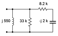
Looking in from the left side, we note that the inductor and 33 k\(\Omega\) resistor are in parallel as they are both tied to the same two nodes. Also, we can see that the capacitor is in series with the 8.2 k\(\Omega\) resistor. This series combination is, in turn, in parallel with the other two parallel components. Thus, it would make sense to find the series combination first.
\[Z_{series} = R+(− jX_C ) \nonumber \]
\[Z_{series} = 8.2 k\Omega − j 2k \Omega \nonumber \]
\[Z_{series} = 8440\angle −13.7^{\circ} \Omega \nonumber \]
We now place this new complex impedance in parallel with the inductor and the 33 k\(\Omega\) resistor.
\[Z_{total} = \frac{1}{\frac{1}{Z_1} + \frac{1}{Z_2} + \frac{1}{Z_3}} \nonumber \]
\[Z_{total} = \frac{1}{\frac{1}{j 550 \Omega} + \frac{1}{33 k\Omega} + \frac{1}{8440\angle −13.7^{\circ} \Omega}} \nonumber \]
\[Z_{total} = 556.8\angle 85.4^{\circ} \Omega \nonumber \]
Clearly, the inductor dominates here. The parallel resistor is roughly two orders of magnitude larger than the inductive reactance and has minimal impact on a parallel combination. Further, the complex impedance derived from the capacitor/resistor combination is also considerably larger, and given that it has a negative (capacitive) phase angle, it partly cancels the inductive reactance. This leaves us with a magnitude a little higher than that of the inductive reactance alone, and with a phase angle shifted toward the resistive side.
The series and parallel combinations can be much more complicated than that of the prior network. Ladder networks, for example, feature a set of sections that load other sections, resulting in repeated series and then parallel simplifications. In this situation, it is best to start work at the end farthest from the nodes of interest. The following example will illustrate this on a modest scale.
Example \(\PageIndex{2}\)
Determine the equivalent impedance of the network shown in Figure \(\PageIndex{2}\).
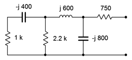
Looking in from the right side, we see immediately the 750 \(\Omega\) resistor. This is in series with the sub-circuit comprised of the remaining five components. This sub-circuit can be seen as the \(−j800 \Omega \) capacitor in parallel with another sub-circuit containing the other four components. This four component subcircuit consists of the inductor in series with yet another sub-circuit consisting of the final two resistors and capacitor. This three element subcircuit consists of the 2.2 k \(\Omega\) resistor in parallel with the series combination of the 1 k\(\Omega\) resistor and the \(−j400 \Omega \) capacitor.
The most sensible way to approach this is to start at the left end with the simple RC series combination and then work right, toward the nodes of interest. We'll number the components from left to right for identification.
\[Z_{left2} = R_1+(− jX_{C1}) \nonumber \]
\[Z_{left2} = 1k \Omega − j 400 \Omega \nonumber \]
\[Z_{left2} = 1077\angle −21.8^{\circ} \Omega \nonumber \]
We now place this complex impedance in parallel with the 2.2 k\(\Omega\) resistor. This creates a three element sub-circuit which is in series with the inductor.
\[Z_{left3} = \frac{1}{\frac{1}{R_2} + \frac{1}{Z_{left2}}} \nonumber \]
\[Z_{left3} = \frac{1}{\frac{1}{2.2 k\Omega} + \frac{1}{1077\angle −21.8^{\circ} \Omega}} \nonumber \]
\[Z_{left3} = 734.7\angle −14.7^{\circ} \Omega \nonumber \]
\[Z_{left4} = Z_{left3} +jX_L \nonumber \]
\[Z_{left4} = 734.7\angle −14.7^{\circ} \Omega +j 600\Omega \nonumber \]
\[Z_{left4} = 822.5\angle 30.2 ^{\circ} \Omega \nonumber \]
This group of four is in parallel with the second capacitor of \(−j800 \Omega \). Finally, we arrive at the equivalent total value by placing the resulting group of five in series with the 750 \(\Omega\) resistor.
\[Z_{left5} = \frac{1}{\frac{1}{X_{C2}} + \frac{1}{Z_{left4}}} \nonumber \]
\[Z_{left5} = \frac{1}{\frac{1}{− j 800 \Omega} + \frac{1}{822.5\angle 30.2^{\circ} \Omega}} \nonumber \]
\[Z_{left5} = 813.4\angle −31.3^{\circ} \Omega \nonumber \]
\[Z_{total} = Z_{left5} +R_3 \nonumber \]
\[Z_{total} = 813.4\angle −31.3^{\circ} \Omega +750 \Omega \nonumber \]
\[Z_{total} = 1506\angle −16.3^{\circ} \Omega \nonumber \]
In rectangular form this is 1443 \(−j422.3 \Omega \), meaning that this network is equivalent to a 1443 \(\Omega\) resistor in series with a capacitive reactance of \(−j422.3 \Omega \).
Series-parallel simplification techniques will not work for all circuits. Some networks such as delta or bridge configurations require other techniques that will be addressed in later chapters.