
7.3: Power Triangle
- Page ID
- 25281

The prior section revealed that the phase angle between the current and voltage cannot be ignored when computing power. For example, if a 120 volt RMS source delivers 2 amps of current, it appears that it delivers 240 watts. This is only true if the load is purely resistive. For a complex load, the true power is somewhat less. In fact, as we've just seen, if the load is purely reactive, there will be no true load power at all.
Although plotting the current, voltage and power waveforms is instructive, it can be somewhat cumbersome. Instead, we use a power triangle as shown in Figure \(\PageIndex{1}\). The horizontal axis represents true power, \(P\), in watts. The vertical axis represents reactive power, \(Q\), in VAR. The vector combination of \(P\) and \(Q\) results in the apparent power, \(S\), in VA. Remember, the apparent power is the product of the magnitudes of the current and voltage. This is what the power “appears to be” based on simple current and voltage measurements from a DMM, versus a proper power meter. In the resistive case, there is no reactive power and thus \(S\) and \(P\) are the same. Consequently, the \(S\) vector collapses onto the \(P\) vector. In a purely reactive case, there is no true power and \(S\) and \(Q\) are the same; both vectors identical and vertical. For the complex case, \(S\) is the vector sum of \(P\) and \(Q\). This simple graphic nicely encapsulates the relationship between the three vectors. Further, given any two of the four parts (three vector magnitudes and \( \theta \)) and with just a little trigonometry, the other two parts may be found.
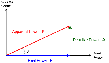
For example, knowing the real and reactive powers, the apparent power can be found via the Pythagorean theorem. Similarly, if the apparent power and angle are known, the real and reactive powers may be found using sine and cosine. Remember, apparent power can be found from the product of the RMS voltage and current magnitudes for any complex impedance, and \( \theta \) is the same as the impedance angle (i.e., the voltage angle minus the current angle). For your convenience, some useful power triangle relationships are listed following.
\[S = v_{RMS} \times i_{RMS} \label{7.4} \]
\[S = \sqrt{P^2+Q^2} \label{7.5} \]
\[\theta = \tan^{-1} \frac{Q}{P} \text{ (i.e., the impedance angle)} \label{7.6} \]
\[P = S \cos \theta \label{7.7} \]
\[P = \sqrt{S^2−Q^2} \label{7.8} \]
\[Q = S \sin \theta \label{7.9} \]
\[Q = \sqrt{S^2−P^2} \label{7.10} \]
Power Factor
As we are often interested in the true power, it is worth noting that a rearrangement of Equation \ref{7.7} shows that the ratio of true power to apparent power is the cosine of the impedance angle, \(P/S = \cos \theta \). This is known as the power factor and is abbreviated \(PF\). Thus, \(PF = \cos \theta\). Knowing the phase angle and the apparent power, true power can be calculated. If \(PF\) is positive it is said to be a lagging power factor. This is the case for inductive loads where the current is lagging the voltage. In contrast, a capacitive load results in a negative or leading \(PF\). Recall that for capacitors, current leads the voltage. The sign is only used to indicate leading or lagging and will be useful when we examine power factor correction, shortly. For example, if a 100 volt RMS source delivers 1 amp for an apparent power of 100 VA and the phase angle is \(−30^{\circ}\), \(PF\) is \(\cos (−30^{\circ})\) or 0.866 leading and the true power is \(P = 100 \cos (−30^{\circ}) = 86.6\) watts.
\[PF = \frac{P}{S} = \cos \theta \text{ (positive is lagging and inductive)} \label{7.11} \]
Example \(\PageIndex{1}\)
Find \(S\), \(P\) and \(Q\) in the circuit of Figure \(\PageIndex{2}\). \(E = 120\) volts RMS. The source frequency is 60 Hz.
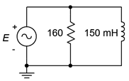
The first step is to determine the inductive reactance.
\[X_L = 2\pi f L \nonumber \]
\[X_L = 2\pi 60 Hz 150 mH \nonumber \]
\[X_L = j 56.55\Omega \nonumber \]
From here we can determine the system impedance which will, in turn, allow us to determine the source current.
\[Z = \frac{R\times jX_L}{R + jX_L} \nonumber \]
\[Z = \frac{160\Omega \times ( j 56.55 \Omega )}{160 \Omega + j56.55\Omega} \nonumber \]
\[Z = 53.3\angle 70.5^{\circ} \Omega \nonumber \]
\[i_{source} = \frac{e_{source}}{Z} \nonumber \]
\[i_{source} = \frac{120\angle 0^{\circ} V}{53.3\angle 70.5^{\circ} \Omega} \nonumber \]
\[i_{source} = 2.252\angle −70.5^{\circ} A \nonumber \]
The apparent power is the product of the magnitudes of circuit voltage and current.
\[S = E\times i_{source} \nonumber \]
\[S = 120 V\times 2.252 A \nonumber \]
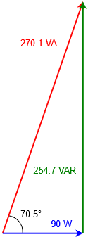
\[S = 270.1 \text{ VA, inductive} \nonumber \]
\[P = S \cos \theta \nonumber \]
\[P = 270.1 VA \cos 70.5^{\circ} \nonumber \]
\[P = 90 W \nonumber \]
\[Q = S \sin \theta \nonumber \]
\[Q = 270.1 VA \sin 70.5^{\circ} \nonumber \]
\[Q = 254.7 \text{ VAR, inductive} \nonumber \]
As a crosscheck, the true power can also be determined by squaring the RMS voltage and then dividing by the 160 \(\Omega \) resistance. Similarly, dividing the squared voltage by \(X_L\) will generate \(Q\).
\[P = \frac{v_R^2}{R} \nonumber \]
\[P = \frac{120 V^2}{160 \Omega} \nonumber \]
\[P = 90 W \nonumber \]
The power triangle for this circuit is shown in Figure \(\PageIndex{3}\).
Power Factor Correction
One issue with a reactive load is that the current is higher than it needs to be in order to achieve a certain true load power. This is wasteful and would require larger conductors. To alleviate these issues, an opposite reactance can be added to the load such that the resulting load is purely resistive. This can be realized by determining the original \(Q\) value and then adding a sufficient reactance to produce an additional \(Q\) of the opposite sign resulting in cancellation. From there, it is short step to determine the required impedance. Then, knowing the frequency, the required capacitance or inductance can then be found using the appropriate reactance formula. This is illustrated in the following example.
Example \(\PageIndex{2}\)
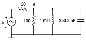
Find circuit \(PF\), \(S\), \(P\) and \(Q\) for Figure \(\PageIndex{4}\). \(E = 20\angle 0^{\circ}\) volts peak at a frequency of 10 kHz. Also find an appropriate component which when placed from node \(a\) to ground brings \(PF\) to unity.
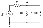
The inductive reactance of 1 mH at 10 kHz is \(j62.83 \Omega \). This is in parallel with the 100 \(\Omega \) resistor, which is then in series with the 20 \(\Omega \) resistor.
\[Z = 20\Omega +(100\Omega || j 62.83\Omega ) \nonumber \]
\[Z = 20\Omega +(28.3+j 45\Omega ) \nonumber \]
\[Z = 66 \angle 43^{\circ} \Omega \nonumber \]
This time we shall use peak values to illustrate the difference compared to using RMS values as in the previous example. The source current is:
\[i_{source} = \frac{E}{Z} \nonumber \]
\[i_{source} = \frac{20\angle 0^{\circ} V}{66\angle 43^{\circ} \Omega} \nonumber \]
\[i_{source} = 0.303\angle −43^{\circ} A \text{ peak} \nonumber \]
To find \(S\), multiply the magnitudes of source voltage and current. As these are peak values, multiply each by 0.707 to arrive at RMS, or just cut the answer in half (i.e., \(0.707^2\) is 0.5). This is the apparent power of the whole circuit.
\[S = \frac{E\times i_{source}}{2} \nonumber \]
\[S = \frac{20 V\times 0.303 A}{2} \nonumber \]
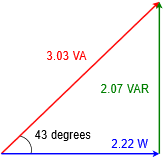
\[S = 3.03 \text{ VA, inductive} \nonumber \]
\[P = S \cos \theta \nonumber \]
\[P = 3.03 VA \cos 43^{\circ} \nonumber \]
\[P = 2.22 W \nonumber \]
To be clear, 2.22 watts is the combined power dissipation between the two resistors.
\[Q = S \sin \theta \nonumber \]
\[Q = 3.03 VA \sin 43^{\circ} \nonumber \]
\[Q = 2.07 \text{ VAR, inductive} \nonumber \]
The power triangle for this circuit is shown in Figure \(\PageIndex{5}\).
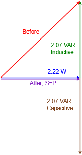
For the second part involving power factor correction, we need to add a reactive power equal in magnitude to the existing value but of the opposite sign. This means we need to add 2.07 VAR capacitive. The new power triangle is shown in Figure \(\PageIndex{6}\). The vertical components cancel, resulting in the apparent power equaling the true power with \(PF = 1\).
We can place the correction capacitor where it's convenient in physical terms, just as long as we add 2.07 VAR capacitive. We don't have a physical circuit, so that's not a consideration here. A convenient location would be to place it across the existing resistor-inductor combo. Our goal then is to first find the required reactance, and from that, determined the required capacitance. We shall do this two different ways. In the first case, we note that the capacitor appears across the only other reactive element in the circuit. Therefore, in order for them to cancel they must have the same reactance magnitude, and thus \(X_C\) must equal \(−j62.8 \Omega\). But what if there were multiple reactive elements in the circuit or if it was impractical to locate the component there, for example, due to space restrictions? In that case, we would simply work the power relation backwards. For comparison, suppose we place the capacitor in the same location; from node \(a\) to ground. A voltage divider can be used to determine the present value of \(v_a\). This works out to 11.4 volts RMS. Using the voltage form of the power rule:
\[Q = \frac{v_X^2}{X} \nonumber \]
\[X = \frac{v_X^2}{Q} \nonumber \]
\[X = \frac{11.4V^2}{2.07VAR} \nonumber \]
\[X = 62.8\Omega \nonumber \]
Either way we derive \(X_C\), now we just solve the capacitive reactance formula to find \(C\).
\[C = \frac{1}{2\pi f X_C} \nonumber \]
\[ C = \frac{1}{2\pi 10 kHz62.8\Omega} \nonumber \]
\[C = 253.3 nF \nonumber \]
The resulting circuit is shown in Figure \(\PageIndex{7}\).
Computer Simulation
It is useful to see the reduction in current demand caused by using power factor correction. To so so, the circuit of Figure \(\PageIndex{7}\) is captured in a simulator as shown in Figure \(\PageIndex{8}\).
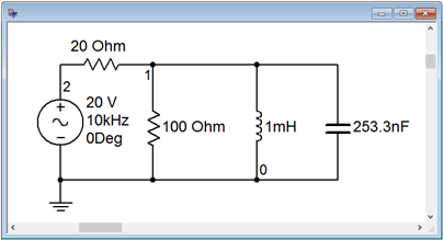
We will run two transient analyses to find the source current. The first version will be run using the original circuit configuration without the capacitor. The second run will include the capacitor. To plot the currents, we will make use of Ohm's law. First we obtain the voltages at nodes 1 and 2. Then, using the simulator's post processor, we subtract \(v_1\) from \(v_2\) which yields the voltage across the 20 \(\Omega \) resistor. This quantity is then divided by 20 \(\Omega \) to arrive at the input current. This is similar to the current sense resistor technique used in earlier chapters.
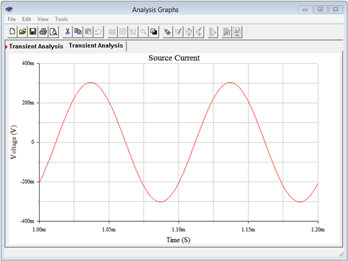
The resulting current for the original circuit is shown in Figure \(\PageIndex{9}\). Note that the peak current is just over 300 milliamps, as calculated in step two of the example.
The second simulation is shown in Figure \(\PageIndex{10}\), now with power factor correction.
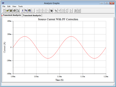
The amplitude here is much reduced, in the range of 160 to 170 milliamps peak. By adding the capacitor, the two reactive currents cancel, leaving a parallel impedance of just 100 \(\Omega \). This is in series with the 20 \(\Omega \) resistor. Dividing 120 \(\Omega \) into the 20 volt peak source yields a peak current of approximately 167 mA, in agreement with the simulation. The cancellation of the reactive currents is also shown by the fact that the source current is no longer out of phase. In Figure \(\PageIndex{10}\) the current waveform is in phase and starts at zero, as expected. This implies a load that is the equivalent of a pure resistance. In contrast, the plot of Figure \(\PageIndex{9}\) shows a current that is lagging by around one-half division, or about 45 degrees, which unsurprisingly is the approximate value of the circuit's impedance angle. Obviously then, this combined impedance must be inductive.
To sum up, power factor correction is used to lower current demand while keeping load power constant. If the load is fixed, this can be achieved through the use of a capacitor (for inductive loads) or an inductor (for capacitive loads). If the load demand is dynamic, then a more complex system is required, for example, switching through a bank of capacitors to get a value close to the precise value needed for that particular load. More examples of power factor correction are in the next section.
References
1Hyperbole seems to work for the movie industry, anyway.