2.8: Antenna Array

An antenna array comprises multiple radiating elements, i.e. individual antennas, and focuses a transmit beam in a desired direction. In Figure \(\PageIndex{3}\) the field pattern in the plane of the earth produced by an array of \(30\) antenna elements arranged horizontally is shown. The fields from each antenna element combined to narrow and strengthen the main beam. Side (or grating) lobes are produced and these will result in some interference but their level here is \(40\text{ dB}\) below that of the main beam. This is another way of managing interference in a cellular system but the direction to the mobile unit must be known. Antenna arrays are used in 4G and 5G. The affect of the array is to increase the power density of the main beam and the density relative to that of an isotropic antenna is called the directional gain of the array, \(D_{\text{Array}}\), and is the product of the antenna gain, \(G_{A}\), of an individual antenna element and the array gain, \(G_{\text{Array}}\):

\[\label{eq:1}D_{\text{Array}}=G_{\text{Array}}G_{A} \]

The maximum value of \(G_{\text{Array}}\) is \(N\) for an \(N\) element array. So the maximum directional gain of the array in \(\text{dBi}\) is

\[\label{eq:2}D_{\text{Array}}|_{\text{dBi}}=G_{A}|_{\text{dBi}}+10\log N \]

2.7.1 Multiple Input, Multiple Output

Multiple input, multiple output (MIMO, pronounced my-moe) technology uses multiple antennas to transmit and receive signals. The MIMO concept was developed in the 1990s [9, 10] and implemented in 4G and 5G, and a variety of WLAN systems. MIMO relies on signals traveling on multiple paths between an array of transmit antennas and an array of receive antennas In MIMO these paths are used to carry more information with each path propagates an image of one transmitted signal (from one antenna) that differs in both amplitude and phase from the images following other paths. Effectively there are multiple connections between each transmit antenna and each receive antenna, see Figure \(\PageIndex{1}\). Here a high-speed data-stream is split into several slower data streams, shown in Figure \(\PageIndex{1}\) as the \(\mathsf{a}\), \(\mathsf{b}\), and \(\mathsf{c}\) bitstreams. The distinct bitstreams are separately modulated and sent from their own transmit antenna, with the constellation diagrams of the transmitted modulated signals labeled \(\mathsf{A}\), \(\mathsf{B}\), and \(\mathsf{C}\). The signals from each of the transmit antenna reaches all of the receive antennas by following different uncorrelated paths.

The output of each receive antenna is a linear combination of the multiple transmitted data streams, with the sampled RF phasor diagrams labeled \(\mathsf{M}\), \(\mathsf{N}\), and \(\mathsf{O}\). (It is not really appropriate to call these constellation diagrams.) That is, each receive antenna has a different linear combination of the multiple images. In effect, the output from each receive antenna can be

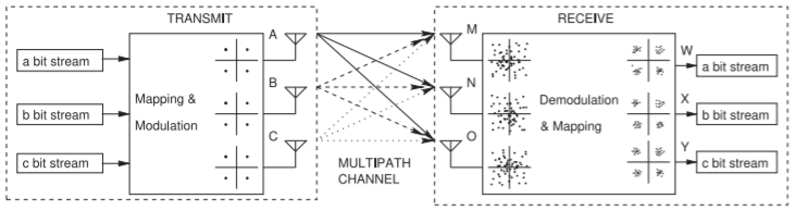
Figure \(\PageIndex{1}\): : A MIMO system showing multiple paths between each transmit antenna and each receive antenna.

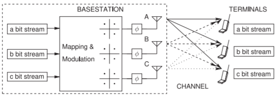
Figure \(\PageIndex{2}\): A massive MIMO system with beams from the basestation antennas to each terminal unit.

thought of as the solution of linear equations, with each transmit antennareceive antenna link corresponding to an equation. Continuing the analogy, the signal from each transmit antenna represents a variable. So a set of simultaneous equations can be solved to obtain the original bitstreams. This is accomplished by demodulation and mapping using knowledge of the channel characteristics to yield the original transmitted signals modified by interference. The result is that the constellation diagrams \(\mathsf{W}\), \(\mathsf{X}\), and \(\mathsf{Y}\) are obtained. The composite channel can be characterized using known test signals.

The capacity of a MIMO system with high SIR scales approximately linearly with the minimum of \(M\) and \(N\), \(\min (M,N)\), where \(M\) is the number of transmit antennas and \(N\) is the number of receive antennas (provided that there is a rich set of paths) [11, 12]. So a system with \(M = N = 4\) will have four times the capacity of a system with just one transmit antenna or one receive antenna.

2.7.2 Massive MIMO

MIMO in 4G uses multiple antennas at the basestation and at the mobile terminals to increase overall data rates provided that there are multiple paths between the transmitter and receiver. In 5G there can be a very large number of transmit antennas even though there are few receive antennas per terminal unit as multiple terminal units mean that there can effectively be a very large number of receive antennas, see Figure \(\PageIndex{2}\).

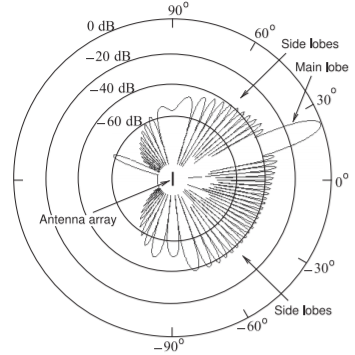
Figure \(\PageIndex{3}\): Electric field pattern from a \(30\) element array of antennas spaced \(0.65\lambda\) apart. The sidelobe levels are about \(40\text{ dB}\) below the power level of the main lobe. The same signal is presented to the antenna elements except that phases of the signal at each antennas is adjusted to produce a main beam directed at \(20\) degrees. The signals to each antenna are thus correlated. After [13].