4.4: Microstrip Transmission Lines

Microstrip has conductors embedded in two dielectric mediums and cannot support a pure TEM mode. In most practical cases, the dielectric substrate is electrically thin, that is, \(h ≪\lambda\). Then the transverse field is dominant and the fields are called quasi-TEM.

4.4.1 Microstrip Line in the Quasi-TEM Approximation

In this section relations are developed based on the principle that the phase velocity of an EM wave in an air-only homogeneous transmission with a TEM field line is just \(c\). As a first step, the potential of the conductor strip is set to \(V_{0}\) and Laplace’s equation is solved using an EM simulator for the electrostatic potential everywhere in the dielectric. Then the per unit length (p.u.l.) electric charge, \(Q\), on the conductor is determined. Using this in the following relation gives the line capacitance:

\[C=\frac{Q}{V_{0}}\nonumber \]

In the next step, the process is repeated with \(\varepsilon_{r} = 1\) to determine \(C_{\text{air}}\) (the capacitance of the line without a dielectric).

If the microstrip line is now an air-filled lossless TEM structure,

\[\label{eq:1} v_{p,\text{air}}=c=\frac{1}{LC_{\text{air}}} \]

and so

\[\label{eq:2} L=\frac{1}{c^{2}C_{\text{air}}} \]

\(L\) is not affected by the dielectric properties of the medium. \(L\) calculated above is the desired p.u.l. inductance of the line with the dielectric as well as in free space. Once \(L\) and \(C\) have been found, the characteristic impedance can be found using

\[\label{eq:3} Z_{0}=\sqrt{\frac{L}{C}} \]

rewritten as

\[\label{eq:4} Z_{0}=\frac{1}{c}\frac{1}{\sqrt{CC_{\text{air}}}} \]

and the phase velocity is

\[\label{eq:5} v_{p}=\frac{1}{\sqrt{LC}}=c\sqrt{\frac{C_{\text{air}}}{C}} \]

Now the field is distributed in the inhomogeneous medium and in free space, as shown in Figure \(\PageIndex{1}\)(a). So the effective relative permittivity, εe, of the equivalent homogeneous microstrip line (see Figure \(\PageIndex{1}\)(b)) is defined by

\[\label{eq:6}\sqrt{\varepsilon_{e}}=\frac{c}{v_{p}} \]

Combining Equations \(\eqref{eq:5}\) and \(\eqref{eq:6}\), the effective relative permittivity (usually just the term effective permittivity is used) is obtained:

\[\label{eq:7}\varepsilon_{e}=\frac{C}{C_{\text{air}}} \]

The effective permittivity can be interpreted as the permittivity of a homogeneous medium that replaces the air and the dielectric regions of the

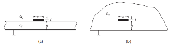
Figure \(\PageIndex{1}\): Microstrip line: (a) cross section; and (b) eps .. equivalent structure where the strip is embedded in a dielectric of semi-infinite extent with effective relative permittivity \(\varepsilon_{e}\).

microstrip, as shown in Figure \(\PageIndex{1}\). Since some of the field is in the dielectric and some is in air, the effective relative permittivity must satisfy

\[\label{eq:8} 1<\varepsilon_{e} <\varepsilon_{r} \]

However, the minimum \(\varepsilon_{e}\) will be greater than \(1\) as electrical energy will be distributed in air and dielectric. The wavelength on a transmission line, the guide wavelength \(\lambda_{g}\), is related to the free space wavelength by \(\lambda_{g} = \lambda_{0}/ \sqrt{\varepsilon_{e}}\).

Example \(\PageIndex{1}\): Microstrip Calculations

A microstrip line has a characteristic impedance \(Z_{0}\) of \(50\:\Omega\) derived from reflection coefficient measurements and an effective permittivity, \(\varepsilon_{e}\), of \(7\) derived from measurement of phase velocity. What is the line’s per-unit-length inductance, \(L\), and capacitance, \(C\)?

Solution

The key equations are \(Z_{0} =\sqrt{L/C}, \varepsilon_{e} = C/C_{\text{air}}\), and in air \(v_{p} = 1/ \sqrt{LC_{\text{air}}} = c\). Also assume that \(\mu_{r} = 1\) which is the default if not specified otherwise and also that \(L\) does not change if only the dielectric is changed. Thus

\[C_{\text{air}}=\frac{C}{\varepsilon_{e}}\quad\text{and then}\quad L=\frac{\varepsilon_{e}}{c^{2}C}\quad\text{so that}\quad Z_{0}=\sqrt{\frac{L}{C}}=\frac{\sqrt{\varepsilon_{e}}}{cC},\quad\text{that is}\quad C=\frac{\sqrt{\varepsilon_{e}}}{cZ_{0}}\nonumber \]

So \(C = \sqrt{7}/(2.998\cdot 10^{8}\times 50) = 1.765\cdot 10^{−10} = 176.5\text{ pF/m}\text{ and }L = Z_{0}^{2}C = 44.13\:\mu\text{H/m}\).

4.4.2 Effective Permittivity and Characteristic Impedance

This section presents formulas for the effective permittivity and characteristic impedance of a microstrip line. These formulas are fits to the results of detailed EM simulations. Also, the form of the equations is based on good physical understanding. First, assume that the thickness, \(t\), is zero. This is not a bad approximation, as \(t ≪ w, h\) for most microwave circuits.

Hammerstad and others provide well-accepted formulas for calculating the effective permittivity and characteristic impedance of microstrip lines [1–3]. Given \(\varepsilon_{r},\: w,\) and \(h\), the effective relative permittivity is

\[\label{eq:9}\varepsilon_{e}=\frac{\varepsilon_{r}+1}{2}+\frac{\varepsilon_{r}-1}{2}\left(1+\frac{10h}{w}\right)^{-a\cdot b} \]

where

\[\label{eq:10} a(u)|_{u=w/h}=1+\frac{1}{49}\ln\left[\frac{u^{4}+\left\{ u/52\right\}^{2}}{u^{4}+0.432}\right] +\frac{1}{18.7}\ln\left[ 1+\left(\frac{u}{18.1}\right)^{3}\right] \]

and

\[\label{eq:11} (\varepsilon_{r} )=0.564\left[\frac{\varepsilon_{r}-0.9}{\varepsilon_{r}+3}\right]^{0.053} \]

Take some time to interpret Equation \(\eqref{eq:9}\), the formula for effective relative permittivity. If \(\varepsilon_{r} = 1\), then \(\varepsilon_{e} = (1 + 1)/2+0 = 1\), as expected. If \(\varepsilon_{r}\) is not that of air, then \(\varepsilon_{e}\) will be between 1 and εr, dependent on the geometry of the line, or more specifically, the ratio \(w/h\). For a very wide line, \(w/h ≫ 1,\: \varepsilon_{e} = (\varepsilon_{r} + 1)/2+(\varepsilon_{r} − 1)/2 = \varepsilon_{r}\), corresponding to the EM energy being confined to the dielectric. For a thin line \(w/h ≪ 1, \varepsilon_{e} = (\varepsilon_{r} + 1)/2\), the average of the dielectric and air permittivities.

Note

Mostly the term “effective permittivity” is used to mean effective relative permittivity (check the magnitude).

The characteristic impedance is given by

\[\label{eq:12} Z_{0}=\frac{Z_{01}}{\sqrt{\varepsilon_{e}}} \]

where the characteristic impedance of the microstrip line in free space is

\[\label{eq:13} Z_{01} =Z_{0}|_{(\varepsilon_{r}=1)}=60\ln\left[\frac{F_{1}h}{w}+\sqrt{1+\left(\frac{2h}{w}\right)^{2}}\right] \]

and

\[\label{eq:14} F_{1}=6+(2\pi -6)\text{exp}\left\{ -(30.666h/w)^{0.7528}\right\} \]

The accuracy of Equation \(\eqref{eq:9}\) is better than \(0.2\%\) for \(0.01 ≤ w/h ≤ 100\) and \(1 ≤ \varepsilon_{r} ≤ 128\). Also, the accuracy of Equation \(\eqref{eq:13}\) is better than \(0.1\%\) for \(w/h < 1000\). Note that \(Z_{0}\) has a maximum value when w is small and a minimum value when w is large.

Now consider the special case where \(w\) is vanishingly small. Then \(\varepsilon_{e}\) has its minimum value:

\[\label{eq:15}\varepsilon_{e}=\frac{1}{2}\left(\varepsilon_{r}+1\right) \]

This leads to an approximate (and convenient) form of Equation \(\eqref{eq:9}\):

\[\label{eq:16}\varepsilon_{e}=\frac{(\varepsilon_{r}+1)}{2}+\frac{(\varepsilon_{r}-1)}{2}\frac{1}{\sqrt{1+12h/w}} \]

This approximation has its greatest error for low and high εr and narrow lines, \(w/h ≪ 1\), where the maximum error is \(1\%\). Again, Equation \(\eqref{eq:12}\) is used to calculate the characteristic impedance. The more exact analysis, represented by Equation \(\eqref{eq:9}\), was used to develop Table \(\PageIndex{1}\), which can be used in the design of microstrip.

Example \(\PageIndex{2}\): Microstrip Characteristic Impedance Calculation

The strip of a microstrip line has a width of \(600\:\mu\text{m}\) and is fabricated on a lossless substrate that is \(635\:\mu\text{m}\) thick and has a relative permittivity of \(4.1\).

1. What is the effective relative permittivity?
2. What is the characteristic impedance?
3. What is the propagation constant at \(5\text{ GHz}\) ignoring any losses?

Solution

Use the formulas for effective permittivity, characteristic impedance, and attenuation constant from Section 4.4.2 with \(w = 600\:\mu\text{m};\: h = 635\:\mu\text{m};\: \varepsilon_{r} = 4.1;\text{ w/h} = 600/635 = 0.945\).

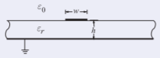
Figure \(\PageIndex{2}\)

1. \[\varepsilon_{e}=\frac{\varepsilon_{r}+1}{2}+\frac{\varepsilon_{r}-1}{2}\left( 1+\frac{10h}{w}\right)^{-a\cdot b}\nonumber \]
   From equations \(\eqref{eq:10}\) and \(\eqref{eq:11}\),
   \[\begin{aligned} a&=1+\frac{1}{49}\ln\left[\frac{(w/h)^{4}+\left\{ w/(52h)\right\} ^{2}}{(w/h)^{4}+0.432}\right]+\frac{1}{18.7}\ln\left[1+\left(\frac{w}{18.1h}\right)^{3}\right] =0.991 \\ b&=0.564 \left[\frac{\varepsilon_{r}-0.9}{\varepsilon_{r}+3}\right]^{0.053}=0.541 \end{aligned} \nonumber \]
   From Equation \(\eqref{eq:9}\), \(\varepsilon_{e}=2.967\)
2. In free space,
   \[Z_{0}|_{\text{air}}=60\ln\left[\frac{F_{1}\cdot h}{w}+\sqrt{1+\left(\frac{2h}{w}\right)^{2}}\right]\nonumber \]
   where \(F_{1}=6 + (2π − 6)\text{ exp}\left\{ − (30.666h/\omega )^{ 0.7528}\right\} ,\quad Z_{0} = Z_{0}|_{\text{air}} /\sqrt{\varepsilon_{e}}\)
   \[Z_{0}|_{\text{air}}=129.7\:\Omega\quad\text{and}\quad Z_{0}=Z_{0}|_{\text{air}} /\sqrt{\varepsilon_{e}}=75.4\:\Omega\nonumber \]
3. \(f=5\text{ GHz},\omega =2\pi f,\:\gamma =\jmath\omega\sqrt{\mu_{0}\varepsilon_{0}\varepsilon_{e}}=\jmath 180.5/\text{ m}\).

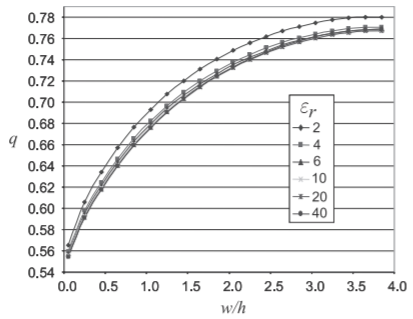
Figure \(\PageIndex{3}\): Dependence of the q factor of a microstrip line at \(1\text{ GHz}\) for various permittivities and aspect (\(\text{w/h}\)) ratios. (Data obtained from EM field simulations using Sonnet.)

4.4.3 Filling Factor

Defining a filling factor, \(q\), provides useful insight into the distribution of energy in an inhomogeneous transmission line. The effective microstrip permittivity is

\[\label{eq:17}\varepsilon_{e}=1+q(\varepsilon_{r}-1) \]

where for a microstrip line \(q\) has the bounds \(\frac{1}{2} ≤ q ≤ 1\) and is almost independent of \(\varepsilon_{r}\). A \(q\) of \(1\) indicates that all of the fields are in the dielectric region. The dependence of the \(q\) of a microstrip line at \(1\text{ GHz}\) for various permittivities and aspect (\(\text{w/h}\)) ratios is shown in Figure \(\PageIndex{3}\). Fitting yields:

\[\label{eq:18} q=\frac{1}{2}\left(1+\frac{1}{\sqrt{1+12h/w}}\right) \]

\(Z_{0}\)	\(\varepsilon_{r} =4\text{ (SiO}_{2}\text{, FR4)}\)		\(\varepsilon_{r}=10\:\text{(Alumina)}\)		\(\varepsilon_{r}=11.9\:\text{(Si)}\)
(\(\Omega \))	\(u\)	\(\varepsilon_{e}\)	\(u\)	\(\varepsilon_{e}\)	\(u\)	\(\varepsilon_{e}\)
\(140\)	\(0.171\)	\(2.718\)	\(0.028\)	\(5.914\)	\(0.017\)	\(6.907\)
\(139\)	\(0.176\)	\(2.720\)	\(0.029\)	\(5.917\)	\(0.018\)	\(6.910\)
\(138\)	\(0.181\)	\(2.722\)	\(0.030\)	\(5.919\)	\(0.019\)	\(6.914\)
\(137\)	\(0.185\)	\(2.723\)	\(0.031\)	\(5.922\)	\(0.020\)	\(6.919\)
\(136\)	\(0.190\)	\(2.725\)	\(0.032\)	\(5.924\)	\(0.021\)	\(6.923\)
\(135\)	\(0.195\)	\(2.727\)	\(0.033\)	\(5.927\)	\(0.022\)	\(6.925\)
\(134\)	\(0.201\)	\(2.729\)	\(0.035\)	\(5.931\)	\(0.022\)	\(6.927\)
\(133\)	\(0.206\)	\(2.731\)	\(0.036\)	\(5.933\)	\(0.023\)	\(6.930\)
\(132\)	\(0.212\)	\(2.733\)	\(0.037\)	\(5.936\)	\(0.024\)	\(6.934\)
\(131\)	\(0.217\)	\(2.734\)	\(0.038\)	\(5.939\)	\(0.025\)	\(6.937\)
\(130\)	\(0.223\)	\(2.736\)	\(0.040\)	\(5.942\)	\(0.026\)	\(6.941\)
\(129\)	\(0.229\)	\(2.738\)	\(0.043\)	\(5.949\)	\(0.028\)	\(6.948\)
\(128\)	\(0.235\)	\(2.740\)	\(0.044\)	\(5.951\)	\(0.029\)	\(6.951\)
\(127\)	\(0.241\)	\(2.742\)	\(0.046\)	\(5.955\)	\(0.030\)	\(6.954\)
\(126\)	\(0.248\)	\(2.744\)	\(0.048\)	\(5.958\)	\(0.031\)	\(6.957\)
\(125\)	\(0.254\)	\(2.746\)	\(0.050\)	\(5.962\)	\(0.033\)	\(6.963\)
\(124\)	\(0.261\)	\(2.748\)	\(0.052\)	\(5.966\)	\(0.034\)	\(6.966\)
\(123\)	\(0.268\)	\(2.750\)	\(0.054\)	\(5.970\)	\(0.035\)	\(6.969\)
\(122\)	\(0.275\)	\(2.752\)	\(0.056\)	\(5.973\)	\(0.038\)	\(6.977\)
\(121\)	\(0.283\)	\(2.755\)	\(0.058\)	\(5.977\)	\(0.039\)	\(6.980\)
\(120\)	\(0.290\)	\(2.757\)	\(0.061\)	\(5.982\)	\(0.041\)	\(6.985\)
\(119\)	\(0.298\)	\(2.759\)	\(0.063\)	\(5.985\)	\(0.043\)	\(6.990\)
\(118\)	\(0.306\)	\(2.761\)	\(0.066\)	\(5.990\)	\(0.045\)	\(6.995\)
\(117\)	\(0.314\)	\(2.763\)	\(0.068\)	\(5.993\)	\(0.047\)	\(6.999\)
\(116\)	\(0.323\)	\(2.766\)	\(0.071\)	\(5.998\)	\(0.049\)	\(7.004\)
\(115\)	\(0.331\)	\(2.768\)	\(0.074\)	\(6.003\)	\(0.051\)	\(7.008\)
\(114\)	\(0.340\)	\(2.771\)	\(0.077\)	\(6.007\)	\(0.053\)	\(7.013\)
\(113\)	\(0.349\)	\(2.773\)	\(0.080\)	\(6.012\)	\(0.055\)	\(7.017\)
\(112\)	\(0.359\)	\(2.776\)	\(0.083\)	\(6.016\)	\(0.057\)	\(7.022\)
\(111\)	\(0.368\)	\(2.778\)	\(0.086\)	\(6.021\)	\(0.060\)	\(7.028\)
\(110\)	\(0.378\)	\(2.781\)	\(0.089\)	\(6.025\)	\(0.062\)	\(7.032\)
\(109\)	\(0.389\)	\(2.783\)	\(0.093\)	\(6.031\)	\(0.065\)	\(7.038\)
\(108\)	\(0.399\)	\(2.786\)	\(0.097\)	\(6.036\)	\(0.068\)	\(7.044\)
\(107\)	\(0.410\)	\(2.789\)	\(0.100\)	\(6.040\)	\(0.071\)	\(7.050\)
\(106\)	\(0.421\)	\(2.791\)	\(0.104\)	\(6.046\)	\(0.074\)	\(7.055\)
\(105\)	\(0.432\)	\(2.794\)	\(0.109\)	\(6.052\)	\(0.077\)	\(7.061\)
\(104\)	\(0.444\)	\(2.797\)	\(0.113\)	\(6.057\)	\(0.080\)	\(7.066\)
\(103\)	\(0.456\)	\(2.800\)	\(0.117\)	\(6.062\)	\(0.084\)	\(7.073\)
\(102\)	\(0.468\)	\(2.803\)	\(0.122\)	\(6.069\)	\(0.087\)	\(7.079\)
\(101\)	\(0.481\)	\(2.806\)	\(0.127\)	\(6.075\)	\(0.091\)	\(7.085\)
\(100\)	\(0.494\)	\(2.809\)	\(0.132\)	\(6.081\)	\(0.095\)	\(7.092\)
\(99\)	\(0.507\)	\(2.812\)	\(0.137\)	\(6.087\)	\(0.099\)	\(7.099\)
\(98\)	\(0.521\)	\(2.815\)	\(0.143\)	\(6.094\)	\(0.103\)	\(7.105\)
\(97\)	\(0.535\)	\(2.819\)	\(0.148\)	\(6.100\)	\(0.108\)	\(7.113\)
\(96\)	\(0.550\)	\(2.822\)	\(0.154\)	\(6.106\)	\(0.112\)	\(7.120\)
\(95\)	\(0.565\)	\(2.825\)	\(0.160\)	\(6.113\)	\(0.117\)	\(7.127\)
\(94\)	\(0.580\)	\(2.829\)	\(0.167\)	\(6.121\)	\(0.122\)	\(7.135\)
\(93\)	\(0.596\)	\(2.832\)	\(0.173\)	\(6.127\)	\(0.128\)	\(7.144\)
\(92\)	\(0.612\)	\(2.836\)	\(0.180\)	\(6.134\)	\(0.133\)	\(7.151\)
\(91\)	\(0.629\)	\(2.839\)	\(0.187\)	\(6.142\)	\(0.139\)	\(7.159\)
\(90\)	\(0.646\)	\(2.843\)	\(0.195\)	\(6.150\)	\(0.145\)	\(7.168\)
\(89\)	\(0.664\)	\(2.847\)	\(0.202\)	\(6.157\)	\(0.151\)	\(7.176\)
\(87\)	\(0.701\)	\(2.855\)	\(0.219\)	\(6.173\)	\(0.164\)	\(7.193\)
\(86\)	\(0.721\)	\(2.859\)	\(0.228\)	\(6.182\)	\(0.171\)	\(7.203\)
\(85\)	\(0.740\)	\(2.863\)	\(0.237\)	\(6.190\)	\(0.179\)	\(7.213\)
\(84\)	\(0.761\)	\(2.867\)	\(0.246\)	\(6.198\)	\(0.187\)	\(7.223\)
\(83\)	\(0.782\)	\(2.872\)	\(0.256\)	\(6.208\)	\(0.195\)	\(7.233\)
\(82\)	\(0.804\)	\(2.876\)	\(0.266\)	\(6.216\)	\(0.203\)	\(7.242\)
\(81\)	\(0.826\)	\(2.881\)	\(0.277\)	\(6.226\)	\(0.212\)	\(7.253\)
\(80\)	\(0.849\)	\(2.885\)	\(0.288\)	\(6.235\)	\(0.221\)	\(7.263\)
\(79\)	\(0.873\)	\(2.890\)	\(0.299\)	\(6.245\)	\(0.230\)	\(7.274\)
\(78\)	\(0.898\)	\(2.895\)	\(0.311\)	\(6.255\)	\(0.240\)	\(7.285\)
\(77\)	\(0.923\)	\(2.900\)	\(0.324\)	\(6.265\)	\(0.251\)	\(7.297\)
\(76\)	\(0.949\)	\(2.905\)	\(0.337\)	\(6.276\)	\(0.262\)	\(7.309\)
\(75\)	\(0.976\)	\(2.910\)	\(0.350\)	\(6.286\)	\(0.273\)	\(7.321\)
\(74\)	\(1.003\)	\(2.915\)	\(0.364\)	\(6.297\)	\(0.285\)	\(7.333\)
\(73\)	\(1.032\)	\(2.921\)	\(0.379\)	\(6.309\)	\(0.297\)	\(7.345\)
\(72\)	\(1.062\)	\(2.926\)	\(0.394\)	\(6.320\)	\(0.310\)	\(7.359\)
\(71\)	\(1.092\)	\(2.932\)	\(0.410\)	\(6.332\)	\(0.323\)	\(7.371\)
\(70\)	\(1.123\)	\(2.937\)	\(0.426\)	\(6.34\)	\(0.338\)	\(7.386\)
\(69\)	\(1.156\)	\(2.943\)	\(0.444\)	\(6.357\)	\(0.352\)	\(7.399\)
\(68\)	\(1.190\)	\(2.949\)	\(0.462\)	\(6.369\)	\(0.368\)	\(7.414\)
\(67\)	\(1.224\)	\(2.955\)	\(0.480\)	\(6.382\)	\(0.384\)	\(7.429\)
\(66\)	\(1.260\)	\(2.961\)	\(0.500\)	\(6.396\)	\(0.400\)	\(7.444\)
\(65\)	\(1.298\)	\(2.968\)	\(0.520\)	\(6.410\)	\(0.418\)	\(7.460\)
\(64\)	\(1.336\)	\(2.974\)	\(0.541\)	\(6.424\)	\(0.436\)	\(7.476\)
\(63\)	\(1.376\)	\(2.980\)	\(0.563\)	\(6.439\)	\(0.455\)	\(7.492\)
\(62\)	\(1.417\)	\(2.987\)	\(0.586\)	\(6.454\)	\(0.475\)	\(7.509\)
\(61\)	\(1.460\)	\(2.994\)	\(0.610\)	\(6.470\)	\(0.496\)	\(7.527\)
\(60\)	\(1.504\)	\(3.001\)	\(0.635\)	\(6.486\)	\(0.518\)	\(7.545\)
\(59\)	\(1.551\)	\(3.008\)	\(0.661\)	\(6.502\)	\(0.541\)	\(7.564\)
\(58\)	\(1.598\)	\(3.015\)	\(0.688\)	\(6.519\)	\(0.564\)	\(7.583\)
\(57\)	\(1.648\)	\(3.022\)	\(0.717\)	\(6.538\)	\(0.589\)	\(7.603\)
\(56\)	\(1.700\)	\(3.030\)	\(0.746\)	\(6.556\)	\(0.616\)	\(7.624\)
\(55\)	\(1.753\)	\(3.037\)	\(0.777\)	\(6.575\)	\(0.643\)	\(7.645\)
\(54\)	\(1.809\)	\(3.045\)	\(0.809\)	\(6.594\)	\(0.672\)	\(7.667\)
\(53\)	\(1.867\)	\(3.053\)	\(0.843\)	\(6.614\)	\(0.702\)	\(7.690\)
\(52\)	\(1.927\)	\(3.061\)	\(0.878\)	\(6.635\)	\(0.733\)	\(7.713\)
\(51\)	\(1.991\)	\(3.069\)	\(0.915\)	\(6.657\)	\(0.766\)	\(7.738\)
\(50\)	\(2.056\)	\(3.077\)	\(0.954\)	\(6.679\)	\(0.800\)	\(7.763\)
\(49\)	\(2.125\)	\(3.086\)	\(0.995\)	\(6.702\)	\(0.837\)	\(7.790\)
\(48\)	\(2.197\)	\(3.094\)	\(1.037\)	\(6.726\)	\(0.875\)	\(7.817\)
\(47\)	\(2.272\)	\(3.103\)	\(1.081\)	\(6.750\)	\(0.914\)	\(7.845\)
\(46\)	\(2.350\)	\(3.112\)	\(1.128\)	\(6.775\)	\(0.956\)	\(7.874\)
\(45\)	\(2.432\)	\(3.121\)	\(1.177\)	\(6.801\)	\(1.000\)	\(7.904\)
\(44\)	\(2.518\)	\(3.131\)	\(1.229\)	\(6.828\)	\(1.047\)	\(7.936\)
\(43\)	\(2.609\)	\(3.140\)	\(1.283\)	\(6.856\)	\(1.096\)	\(7.968\)
\(42\)	\(2.703\)	\(3.150\)	\(1.340\)	\(6.884\)	\(1.147\)	\(8.002\)
\(41\)	\(2.803\)	\(3.160\)	\(1.400\)	\(6.913\)	\(1.201\)	\(8.036\)
\(40\)	\(2.908\)	\(3.171\)	\(1.464\)	\(6.944\)	\(1.259\)	\(8.072\)
\(39\)	\(3.019\)	\(3.181\)	\(1.531\)	\(6.974\)	\(1.319\)	\(8.108\)
\(38\)	\(3.136\)	\(3.192\)	\(1.602\)	\(7.006\)	\(1.384\)	\(8.147\)
\(37\)	\(3.259\)	\(3.203\)	\(1.677\)	\(7.039\)	\(1.452\)	\(8.186\)
\(36\)	\(3.390\)	\(3.214\)	\(1.757\)	\(7.073\)	\(1.524\)	\(8.226\)
\(35\)	\(3.528\)	\(3.226\)	\(1.841\)	\(7.108\)	\(1.600\)	\(8.268\)
\(34\)	\(3.675\)	\(3.237\)	\(1.931\)	\(7.143\)	\(1.682\)	\(8.311\)
\(33\)	\(3.831\)	\(3.250\)	\(2.027\)	\(7.180\)	\(1.769\)	\(8.355\)
\(32\)	\(3.997\)	\(3.262\)	\(2.129\)	\(7.218\)	\(1.862\)	\(8.402\)
\(31\)	\(4.174\)	\(3.275\)	\(2.238\)	\(7.258\)	\(1.961\)	\(8.449\)
\(30\)	\(4.364\)	\(3.288\)	\(2.355\)	\(7.298\)	\(2.067\)	\(8.498\)
\(29\)	\(4.567\)	\(3.301\)	\(2.480\)	\(7.340\)	\(2.181\)	\(8.549\)
\(28\)	\(4.875\)	\(3.315\)	\(2.615\)	\(7.384\)	\(2.304\)	\(8.601\)
\(27\)	\(5.020\)	\(3.329\)	\(2.760\)	\(7.428\)	\(2.436\)	\(8.655\)
\(26\)	\(5.273\)	\(3.344\)	\(2.917\)	\(7.475\)	\(2.579\)	\(8.712\)
\(25\)	\(5.547\)	\(3.359\)	\(3.087\)	\(7.523\)	\(2.734\)	\(8.770\)
\(24\)	\(5.845\)	\(3.374\)	\(3.272\)	\(7.573\)	\(2.902\)	\(8.831\)
\(23\)	\(6.169\)	\(3.390\)	\(3.474\)	\(7.625\)	\(3.086\)	\(8.894\)
\(22\)	\(6.523\)	\(3.407\)	\(3.694\)	\(7.679\)	\(3.287\)	\(8.960\)
\(21\)	\(6.912\)	\(3.424\)	\(3.936\)	\(7.734\)	\(3.508\)	\(9.028\)
\(20\)	\(7.341\)	\(3.441\)	\(4.203\)	\(7.793\)	\(3.752\)	\(9.100\)
\(19\)	\(7.815\)	\(3.459\)	\(4.499\)	\(7.854\)	\(4.022\)	\(9.174\)
\(18\)	\(8.344\)	\(3.478\)	\(4.829\)	\(7.917\)	\(4.323\)	\(9.252\)
\(17\)	\(8.936\)	\(3.497\)	\(5.199\)	\(7.983\)	\(4.661\)	\(9.334\)
\(16\)	\(9.603\)	\(3.517\)	\(5.616\)	\(8.053\)	\(5.043\)	\(9.419\)
\(15\)	\(10.361\)	\(3.538\)	\(6.090\)	\(8.126\)	\(5.476\)	\(9.509\)
\(14\)	\(11.229\)	\(3.559\)	\(6.633\)	\(8.202\)	\(5.972\)	\(9.604\)
\(13\)	\(12.233\)	\(3.581\)	\(7.262\)	\(8.282\)	\(6.547\)	\(9.704\)
\(12\)	\(13.407\)	\(3.604\)	\(7.997\)	\(8.367\)	\(7.219\)	\(9.809\)
\(11\)	\(14.798\)	\(3.628\)	\(8.868\)	\(8.456\)	\(8.016\)	\(9.920\)
\(10\)	\(16.471\)	\(3.652\)	\(9.916\)	\(8.550\)	\(8.975\)	\(10.038\)

Table \(\PageIndex{1}\): Microstrip line normalized width \(u (= w/h)\) and effective permittivity, \(\varepsilon_{e}\), for specified characteristic impedance \(Z_{0}\). Data derived from the analysis in Section 4.4.2.