5.3: Multimoding on Transmission Lines

Last updated
Save as PDF

Page ID: 41285

\( \newcommand{\vecs}[1]{\overset { \scriptstyle \rightharpoonup} {\mathbf{#1}} } \) \( \newcommand{\vecd}[1]{\overset{-\!-\!\rightharpoonup}{\vphantom{a}\smash {#1}}} \)\(\newcommand{\id}{\mathrm{id}}\) \( \newcommand{\Span}{\mathrm{span}}\) \( \newcommand{\kernel}{\mathrm{null}\,}\) \( \newcommand{\range}{\mathrm{range}\,}\) \( \newcommand{\RealPart}{\mathrm{Re}}\) \( \newcommand{\ImaginaryPart}{\mathrm{Im}}\) \( \newcommand{\Argument}{\mathrm{Arg}}\) \( \newcommand{\norm}[1]{\| #1 \|}\) \( \newcommand{\inner}[2]{\langle #1, #2 \rangle}\) \( \newcommand{\Span}{\mathrm{span}}\) \(\newcommand{\id}{\mathrm{id}}\) \( \newcommand{\Span}{\mathrm{span}}\) \( \newcommand{\kernel}{\mathrm{null}\,}\) \( \newcommand{\range}{\mathrm{range}\,}\) \( \newcommand{\RealPart}{\mathrm{Re}}\) \( \newcommand{\ImaginaryPart}{\mathrm{Im}}\) \( \newcommand{\Argument}{\mathrm{Arg}}\) \( \newcommand{\norm}[1]{\| #1 \|}\) \( \newcommand{\inner}[2]{\langle #1, #2 \rangle}\) \( \newcommand{\Span}{\mathrm{span}}\)\(\newcommand{\AA}{\unicode[.8,0]{x212B}}\)

Multimoding on a transmission line occurs when there are two or more EM field configurations that can support a propagating wave. Different field configurations travel at different speeds so that the information traveling in two modes will combine randomly and it will be impossible to discern the intended signal. It is critical that the dimensions of a transmission line be small enough to avoid multimoding. Larger dimensions however are more easily manufactured. With microstrip the quasi-TEM mode is supported from DC. Other modes can propagate above a cut-off frequency when transverse dimensions are larger than a quarter or half of a wavelength.

The important concept from EM throry is that electric and magnetic walls in the transverse direction (perpendicular to the direction of propagation) impose boundary conditions on the fields.

5.3.1 Multimoding and Electric and Magnetic Walls

The introduction of a magnetic wall greatly aids in the intuitive understanding of multimoding and in identifying problem situations. A magnetic wall can only be approximated since magnetic charges do not exist. An electric wall requires that the \(E\) field be perpendicular and the \(H\) field be parallel to the wall, see Figure \(\PageIndex{1}\). Similarly a magnetic wall requires that the \(H\) field be perpendicular and the \(E\) field be parallel to the wall, see Figure \(\PageIndex{2}\). A magnetic wall is approximated at the interface of the dielectric and air, see Figure \(\PageIndex{3}\)(a), and near the edges of the strip, see Figure \(\PageIndex{3}\)(b). The electric and magnetic walls establish boundary conditions for Maxwell’s equations with the lowest frequency solutions shown in Table \(\PageIndex{1}\). With two electric or two magnetic walls, a TEM mode (having no field variations in the transverse plane) can be supported. Modes (other than TEM) with geometric variations in the transverse plane have a critical wavelength, \(\lambda_{c}\), and hence a critical frequency, \(f_{c}\), below which the mode cannot propagate. In Figure \(\PageIndex{4}\) the distance between the walls is \(d\). For the case of two like walls (Figures \(\PageIndex{4}\)(a and c)), \(\lambda_{c} = 2h\), as one-half sinusoidal variation is required. With unlike walls (see Figure \(\PageIndex{4}\)(b)), the varying modes are supported with just one-quarter sinusoidal variation, and so \(\lambda_{c} = 4h\).

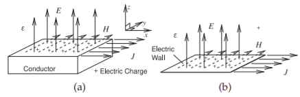
Figure \(\PageIndex{1}\): Properties of an electric wall: (a) the electrical field is perpendicular to a conductor and the magnetic field is parallel to it; and (b) a conductor can be approximated by an electric wall.

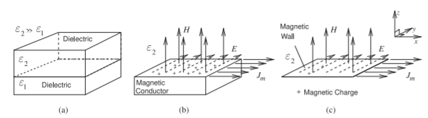
Figure \(\PageIndex{2}\): Properties of the EM field at a magnetic wall: (a) the interface of two dielectrics of contrasting permittivities approximates a magnetic wall; (b) the dielectric with lower permittivity can be approximated as a magnetic conductor; and (c) a magnetic wall.

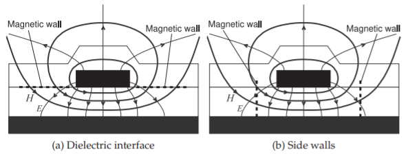
Figure \(\PageIndex{3}\): Approximate magnetic walls in microstrip where the \(H\) field is almost normal and the \(E\) field is almost parallel to the wall.

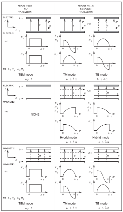
Figure \(\PageIndex{4}\): Lowest-order modes supported by combinations of electric and magnetic walls.

Example \(\PageIndex{1}\): Modes and Electric and Magnetic Walls

A magnetic wall and an electric wall are \(1\text{ cm}\) apart and are separated by a lossless material having \(\varepsilon_{r} = 9\). What is the cut-off frequency of the lowest-order mode in this system?

Solution

The EM field established by the electric and magnetic walls is described in Figure \(\PageIndex{4}\)(b). There is no solution to the Maxwell’s equations that has no variation of the EM fields since it is not possible to have a spatially uniform electric field which is perpendicular to an electric wall while also being perpendicular to a parallel magnetic wall. The other solutions of Maxwell’s equations require that the fields vary spatially, i.e. curl. Without electric and magnetic walls the minimum distance over which the EM fields will fold back on to themselves is a wavelength. With parallel electric and magnetic wall separated by \(h\) the minimum distance for a solution of Maxwell’s equations is a quarter wavelength, \(\lambda\), of the walls as shown on the right in Figure \(\PageIndex{4}\)(b). That is

\[\label{eq:1}h=\lambda /4\quad\text{or}\quad\lambda =4h=4\text{ cm}=\lambda_{0}/(\sqrt{\varepsilon_{t}\mu_{r}}) \]

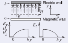
Figure \(\PageIndex{5}\)

Since the relative permeability has not been specified we assume that \(\mu_{r} = 1\) so

\[\lambda_{0}=\lambda\sqrt{9}=12\text{ cm}=c/f\nonumber \]

The cut-off frequency is

\[\begin{align}f&=(2.998\times 10^{8}\text{ m/s})/(0.12\text{ m})\nonumber \\ \label{eq:2}&=2.498\text{ GHz}\end{align} \]