7.2: Two-Port Networks

In microwave circuits it is generally difficult to do this. Recall that with transmission lines it is not possible to establish a common ground point. However, with transmission lines it was seen that for each signal current there is a signal return current. Thus at radio frequencies, and for circuits that are distributed, ports are used, as shown in Figure \(\PageIndex{1}\)(a), which define the voltages and currents for a two-port network, or just two-port.\(^{1}\) The network in Figure \(\PageIndex{1}\)(a) has four terminals and two ports. A port voltage is defined as the voltage difference between a pair of terminals with one of the terminals in the pair becoming the reference terminal. The current entering the network at the top terminal of Port 1 is \(I_{1}\) and there is an equal current leaving the reference terminal. This arrangement clearly makes sense when transmission lines are attached to Ports 1 and 2, as in Figure \(\PageIndex{1}\)(b). With transmission lines at Ports 1 and 2 there will be traveling-wave voltages, and at the ports the traveling-wave components add to give the total port voltage. In dealing with non-distributed circuits it is preferable to use the total port voltages and currents—\(V_{1},\: I_{1},\: V_{2},\) and \(I_{2}\), shown in Figure \(\PageIndex{1}\)(a). However, with distributed elements it is preferable to deal with traveling voltages and currents—\(V_{1}^{+},\:V_{1}^{-},\:V_{2}^{+}\), and \(V_{2}^{-}\), shown in Figure \(\PageIndex{1}\)(b). RF and microwave design necessarily requires switching between the two forms.

7.2.1 Reciprocity, Symmetry, Passivity, and Linearity

Reciprocity, symmetry, passivity, and linearity are fundamental properties of networks. A network is linear if the response is linearly dependent on the drive level, and superposition also applies. So if the two-port shown in Figure \(\PageIndex{1}\)(a) is linear, the currents \(I_{1}\) and \(I_{2}\) are linear functions of \(V_{1}\) and \(V_{2}\). An example of a linear network would be one with resistors and capacitors. A network with a diode would be nonlinear. A passive network has no internal sources of power and a symmetrical two-port has the same characteristics at each of the ports. An example of a symmetrical network is a transmission line with a uniform cross section.

A reciprocal two-port has a response at Port 2 from an excitation at Port 1 that is the same as the response at Port 1 to the same excitation at Port 2. As an example, consider the two-port in Figure \(\PageIndex{1}\)(a) with \(V_{2} = 0\). If the network is reciprocal, then the ratio \(I_{2}/V_{1}\) with \(V_{2} = 0\) will be the same as the ratio \(I_{1}/V_{2}\) with \(V_{1} = 0\). Networks with resistors, capacitors, and transmission lines are reciprocal. A transistor amplifier is not reciprocal as gain is in one direction.

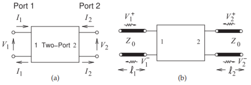
Figure \(\PageIndex{1}\): A twoport network: (a) port voltages; and (b) with transmission lines at the ports.

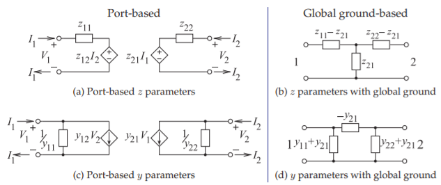
Figure \(\PageIndex{2}\): The \(z\)- and \(y\)-parameter equivalent circuits for port-based and global ground representations. The immittances are shown as impedances.

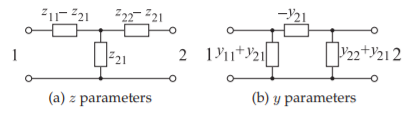
Figure \(\PageIndex{3}\): Circuit equivalence of the \(z\) and \(y\) parameters for a reciprocal network (in (b) the elements are admittances).

7.2.2 Parameters Based on Total Voltage and Current

Here port-based impedance (\(z\)), admittance (\(y\)), and hybrid (\(h\)) parameters will be described. These are similar to the more conventional \(z,\: y,\) and \(h\) parameters defined with respect to a common or global ground. The contrasting circuit representations of the parameters are shown in Figure \(\PageIndex{2}\).

Impedance Parameters

With reference to Figure \(\PageIndex{1}\) the port-based impedance parameters, or \(z\) parameters, are defined as

\[\label{eq:1}V_{1}=z_{11}I_{1}+z_{12}I_{2} \]

\[\label{eq:2}V_{2}=z_{21}I_{1}+z_{22}I_{2} \]

or in matrix form as

\[\label{eq:3}\mathbf{V}=\mathbf{ZI} \]

The double subscript on a parameter is ordered so that the first refers to the output and the second refers to the input, so \(z_{ij}\) relates the voltage output at Port \(i\) to the current input at Port \(j\). If the network is reciprocal, then \(z_{12} = z_{21}\), but this simple type of relationship does not apply to all network parameters. The reciprocal circuit equivalence of the \(z\) parameters is shown in Figure \(\PageIndex{3}\)(a).

Example \(\PageIndex{1}\): Thevenin equivalent of a source with a two-port

What is the Thevenin equivalent circuit of the source-terminated two-port network on the right.

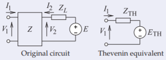
Figure \(\PageIndex{4}\)

Solution

From the original circuit

\[\label{eq:4}V_{1}=Z_{11}I_{1}+Z_{12}I_{2} \]

\[\label{eq:5}V_{2}=Z_{21}I_{1}+Z_{22}I_{2} \]

\[\label{eq:6}V_{2}=E-I_{2}Z_{L} \]

Substituting Equation \(\eqref{eq:6}\) in Equation \(\eqref{eq:5}\)

\[\label{eq:7}E=Z_{21}I_{1}+(Z_{22}+Z_{L})I_{2} \]

Multiplying Equation \(\eqref{eq:4}\) by \((Z_{22} + Z_{L})\) and

Equation \(\eqref{eq:7}\) by \(Z_{12}\)

\[\label{eq:8}(Z_{22}+Z_{L})V_{1}=(Z_{22}+Z_{L})Z_{11}I_{1}+(Z_{22}+Z_{L})Z_{12}I_{2} \]

\[\label{eq:9}Z_{12}E=Z_{12}Z_{21}I_{1}+Z_{12}(Z_{22}+Z_{L})I_{2} \]

Subtracting Equation \(\eqref{eq:9}\) from Equation \(\eqref{eq:8}\)

\[(Z_{22} + Z_{L})V_{1} − Z_{12}E = [(Z_{22} + Z_{L})Z_{11}−]I_{1}\nonumber \]

\[\label{eq:10}V_{1}=\frac{Z_{12}E}{Z_{22}+Z_{L}}+\left(Z_{11}-\frac{Z_{12}Z_{21}}{Z_{22}+Z_{L}}\right)I_{1} \]

For the Thevenin equivalent circuit \(V_{1} = E_{TH} + I_{1}Z_{TH}\) and so

\[\label{eq:11}Z_{TH}=\left(Z_{11}-\frac{Z_{12}Z_{21}}{Z_{22}+Z_{L}}\right)\quad\text{and}\quad E_{TH}=\frac{Z_{12}E}{Z_{22}+Z_{L}} \]

Admittance Parameters

The port-based admittance parameters, or \(y\) parameters, are defined as

\[\label{eq:12}I_{1}=y_{11}V_{1}+y_{12}V_{2} \]

\[\label{eq:13}I_{2}=y_{21}V_{1}+y_{22}V_{2} \]

or in matrix form as

\[\label{eq:14}\mathbf{I}=\mathbf{YV} \]

Now, for reciprocity, \(y_{12} = y_{21}\) and the circuit equivalence of the \(y\) parameters is shown in Figure \(\PageIndex{3}\)(b).

Footnotes

[1] Even when the term “two-port” is used on its own, the hyphen is used, as it is referring to a two-port network.